Symmetric Linear regression?
Often times, we wish to fit a line to data. For many of us, the first method that springs to mind is least squares. But what exactly is the “correct” least squares test? This post will tackle the simple case of a line in 2D, which can be generalized to higher dimensions quite trivially. After discussing the simple case of scattered data with no associated uncertainties, I will extend the results to scenarios where each data point is assumed to be drawn from a Gaussian distribution.
The script for generating the plots in this post is available on GitHub.
2D linear regression
Consider a case where we have $N$ 2D data points, $\boldsymbol{X}=\{x_i, y_i \}_{i=1}^N $, and we believe that they should scatter along the line $\ell=\{ \{x,y\} \,: \, y=ax+b \} $. A straightforward approach might lead us to formulate the sum of squares as follows:
\[S_{\rm naive}=\sum_{i=1}^N\left(ax_i+b-y_i\right)^2.\]Minimizing this with respect to $a$ and $b$ provides a (perhaps familiar) result:
\[a_{\rm opt}=\frac{\sum_{i=1}^N(x_i-\bar{x})^2}{\sum_{i=1}^N(x_i-\bar{x})(y_i-\bar{y})}\;\;,\;\;b_{\rm opt}=\bar{y}-a_{\rm opt}\bar{x},\]where $\bar{y}$ and $\bar{x}$ represent the mean of $y$ and $x$, respectively.
“The ‘challenge’ with this approach is that it treats $x$ and $y$ unequally. Essentially, it computes the sum of distances along the $y$ axis between $y_i$ and $ax_i+b$. Depending on the specific context, this may indeed be the right question. However, in many cases, we might be more interested in a geometrical question. Specifically, we might want to know the sum of distances of the points $\boldsymbol{X}_i$ from the line $\ell$.” To illustrate the ‘challenge’, let’s consider the ‘transposed’ question. We can rewrite the line equation as $\ell={ {x,y} ,: , x=(y-b)/a } $. Following the same logic as before, one might say “the best fit line $x=(y-b)/a$ is the one minimizing $\left(x-y/a +b/a\right)^2$.” This approach, however, minimizes the distance along the x-axis, a distinctly different problem than our original y-axis minimization. Following a simple calculation, the optimal parameters for this ‘transposed’ question are
\[a_{\rm opt}=\frac{\sum_{i=1}^N(x_i-\bar{x})(y_i-\bar{y})}{\sum_{i=1}^N(y_i-\bar{y})^2}\;\;,\;\;b_{\rm opt}=\bar{y}-a_{\rm opt}\bar{x}.\]When we compare this with our earlier result, we see the parameters are different. This result brings us to an important question - should we be minimizing the distance in any specific direction, or is there a more geometrically symmetrical approach? This is precisely the question that we address next.
What’s the Distance Between a Point and a Line??
Ideally, answering such a geometric question should not depend on a specific choice of coordinates. As such, we’d expect the distance to be represented as an inner (or dot) product of $X$ with some vector. Now, you might recall that a line in 2D can be represented by $\hat{\boldsymbol{n}}\cdot\boldsymbol{X}=\alpha$, where $\hat{\boldsymbol{n}}$ is the line’s normal vector, and $\alpha$ determines a specific line from the infinite set of lines perpendicular to $\hat{\boldsymbol{n}}$. By dividing the line equation by $\alpha$, we can normalize it, resulting in:
\[\ell: \{\boldsymbol{X}|\boldsymbol{w}\cdot\boldsymbol{X}=1\}\]While this may be familiar to some, it’s worth detailing a short derivation of the distance between a line and a point, as we’ll soon try to extend this distance concept. We’re interested in finding the point $\boldsymbol{Y}$ that is closest to $\boldsymbol{X}$ and satisfies $\boldsymbol{Y}\cdot\boldsymbol{w}=1$. This can be done by using a Lagrange multiplier $\lambda$, and minimizing the following objective function:
\[D^2=\min_{\boldsymbol{Y}}\vert\boldsymbol{X}-\boldsymbol{Y}\vert^2-2\lambda(\boldsymbol{Y}\cdot\boldsymbol{w}-1)=2\lambda(1-\boldsymbol{w}\cdot\boldsymbol{X})-\lambda^2w^2.\]By requiring that the derivative with respect to $\lambda$ vanishes (to impose the constraint), we find $\lambda=(1-\boldsymbol{w}\cdot\boldsymbol{X})/w^2$. Substituting this back into our objective function, we obtain:
\[D=\frac{\vert\boldsymbol{w}\cdot\boldsymbol{X}-1\vert}{|\boldsymbol{w}|}.\]A more familiar form of this equation is $\vert{\hat{\boldsymbol{n}}}\cdot\boldsymbol{X}’-\alpha\vert$, which matches the above equation if we identify $\alpha=1/w^2$. Hence, the total sum of squares in our scenario is:
\[\boxed{S=\frac{1}{w^2}\sum_i\left(\boldsymbol{w}\cdot\boldsymbol{X}_i-1\right)^2}\]In 2D, this equation reduces to $1=w_xx+w_yy$, or equivalently $y=-w_xx/w_y+1/w_y$. Let’s rename $w_x$ and $w_y$ so that the line equation becomes $y=ax+b$. Our sum of squares then transforms to:
\[S=\frac{1}{1+a^2}\sum_i\left(ax_i+b-y_i\right)^2.\]Minimizing this over $b$ yields a simple expression
\[S_{a}=\frac{1}{1+a^2}\sum_i\left[a(x_i-\bar{x})-(y_i-\bar{y})\right]^2.\]But this time, our optimal $a$ value is different:
\[a_{\rm opt}=\frac{\sum_{i=1}^N(y_i-\bar{y})}{\sum_{i=1}^N(x_i-\bar{x})}\;\;,\;\;b_{\rm opt}=\bar{y}-a_{\rm opt}\bar{x}.\]This final step, minimizing the ‘symmetric’ sum of squared distances, is not as straightforward to generalize to higher dimensions, due to the non-linear nature of $S$ which persists regardless of how we parametrize the line (or surface in higher dimensions).
Let’s denote $\overline{\delta x}=\sum_i (x_i-\bar{x})/N$ and $\overline{\delta y}=\sum_i (y_i-\bar{y})/N$. Using these definitions and our optimal parameters, we can express $\boldsymbol{w}$ as:
\[\boldsymbol{w}=\frac{(\overline{\delta y},-\overline{\delta x})^T}{\bar{x}\overline{\delta x}-\bar{y}\overline{\delta y}},\]This makes the $x\leftrightarrow y$ symmetry explicit: if we swap $x$ and $y$, we also swap $w_x$ and $w_y$. This emphasizes our shift from a one-directional distance measure to a more symmetrical, geometric measure.
In the following figure, we’ve plotted some synthetic data along with the best fit lines according to the different distance measures discussed. These are the $X$ direction, $Y$ direction, and orthogonal distances. You can see that each method yields a distinctly different result. This underlines the fact that the ‘distance’ we choose to minimize can have a significant influence on the line of best fit. Therefore, our choice of distance measure shouldn’t be arbitrary but carefully aligned with the geometrical essence of our problem.
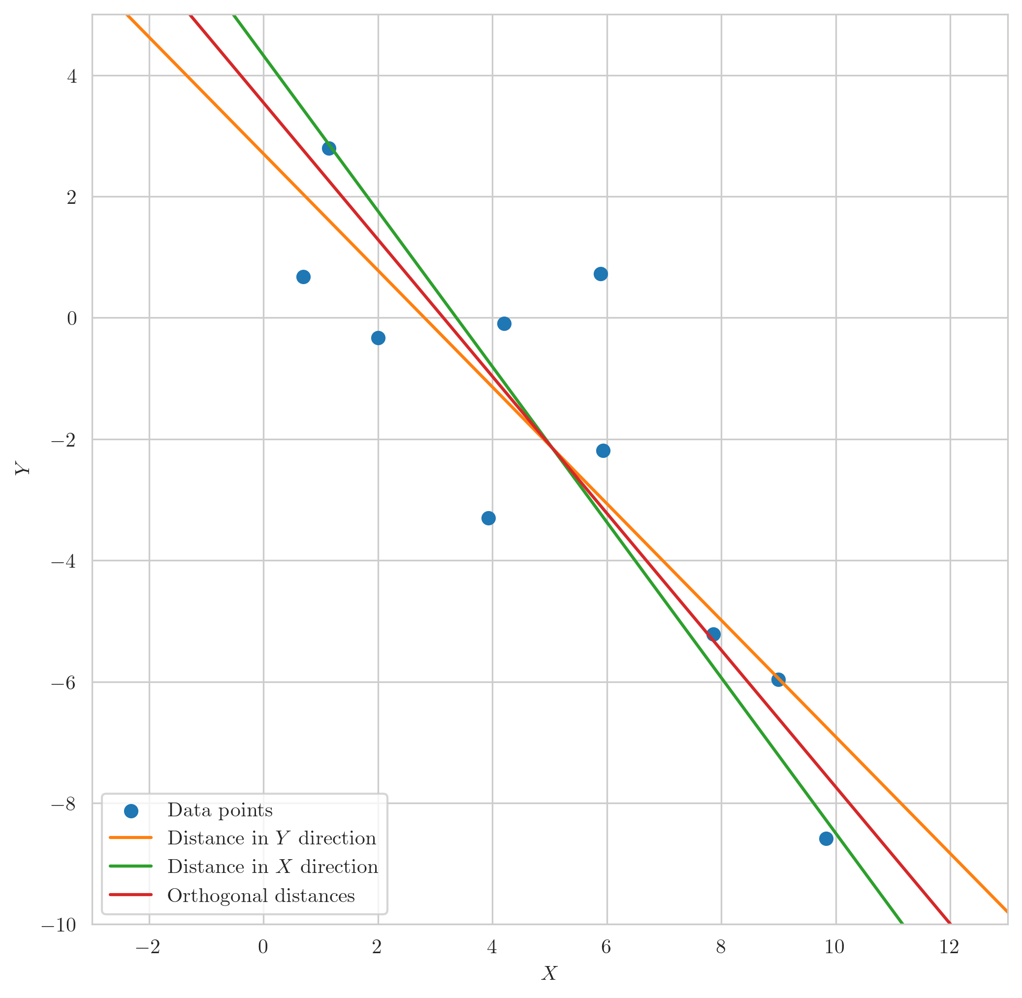 Scatter plot of data points and corresponding lines of best fit computed by minimizing distances in the $Y$ direction (orange), $X$ direction (green), and orthogonal distances (red).
Weighted distance with correlated errors.
The motivation for exploring a symmetrized square distance measure arises from the following scenario. Consider a scenario where we have $N$ data points $\boldsymbol{X}_i$, each measured with a certain level of uncertainty. We model this by assuming each point is sampled from a different normal distribution,
\[\boldsymbol{X}_i\sim{\cal N}(\boldsymbol{\mu}_i,S_i),\]where $S_i$ is the covariance matrix. If we want to find the best linear model that describes the data, we’re looking for a weight vector $\boldsymbol{w}$ such that the data best aligns with $\boldsymbol{w}\cdot\boldsymbol{X}=1$. But, how should we formulate our loss function in this scenario? Specifically, how should we weight each data point considering its correlated errors? This leads us to a critical question - how should we define the distance between a surface and a normal distribution?
The Distance between a Point and a Normal Distribution
The distance between a point and a normal distribution is referred to as theMahalanobis distance. The simplest way to understand this concept is to consider the case of a standard normal distribution, ${\cal N}(\boldsymbol{0},{\mathbb{1}})$. In this case, the Mahalanobis distance is simply the $L_2$ norm. This is intuitive as, in this case, the distribution is symmetric, and the natural distance scale defined by the covariance matrix is set to 1.
Next, recall that if $\boldsymbol{X}\sim{\cal N}(\boldsymbol{\mu},S)$, we can define a new variable $\boldsymbol{Z}\sim{\cal N}(\boldsymbol{0},1)$ using the linear transformation
\[\boldsymbol{Z}=M(\boldsymbol{X}-\boldsymbol{\mu})\;\;,\;\;M^TM=S^{-1}.\]Since $S$ is a positive definite matrix, we know that such a matrix $M$ exists. As the distance in the $Z$ coordinates is simply given by $\vert \boldsymbol{Z}\vert$, the Mahalanobis distance (squared) in the original $\boldsymbol{X}$ coordinates is
\[D_M^2(\boldsymbol{X}; \boldsymbol{\mu},S)=(\boldsymbol{X}-\boldsymbol{\mu})^TS^{-1}(\boldsymbol{X}-\boldsymbol{\mu})\]The Distance between a Surface and a Distribution
Now that we have defined the distance between a point and a distribution, we can utilize it to determine the distance between the distribution and a surface. To do this, we follow identical steps to those we used when looking for the distance between a line (or a surface) and a point. Namely, we seek the point $\boldsymbol{Y}$ closest to the distribution, subject to the constraint $\boldsymbol{w}\cdot\boldsymbol{Y}=1$. We impose this constraint using Lagrange multipliers, leading us to define the following objective function
\[D_{\ell}^2=\min_{\boldsymbol{Y}} (\boldsymbol{Y}-\boldsymbol{\mu})^TS^{-1}(\boldsymbol{Y}-\boldsymbol{\mu})-2\lambda(\boldsymbol{w}\cdot\boldsymbol{Y}-1).\]Setting the derivative with respect to $\boldsymbol{Y}$ equal to zero gives
\[0=2S^{-1}(\boldsymbol{Y}-\boldsymbol{\mu})-2\lambda\boldsymbol{w}\;\;\Rightarrow\;\;\boldsymbol{Y}=\boldsymbol{\mu}+\lambda S\boldsymbol{w},\]so we need to find the extreme point of
\[D_{\ell}=2\lambda(1-\boldsymbol{w}\cdot\boldsymbol{\mu})-\lambda^2\boldsymbol{w}^TS\boldsymbol{w},\]which is given by
\[D_{\ell}^2(\boldsymbol{\mu},S)=\frac{(1-\boldsymbol{w}\cdot \boldsymbol{\mu})^2}{\boldsymbol{w}^TS\boldsymbol{w}}.\]This result is very similar to the known result for the distance from a surface to a point, but with the correct weighting by the covariance matrix to represent measurement uncertainty. Focusing on a line in 2D and replacing $w_x=-a/b\;,\;w_y=1/b$, we can express $D_\ell$ as
\[D_{\ell}^2=\frac{(a x+b-y)^2}{(a,-1)^TS(a,-1)}.\]The above result gives us a way to express the distance from a line to a point in the presence of uncertainties and correlation of variables. To find the best fit parameters for our line, we can define a total sum of Mahalanobis distance squared:
\[S_{M}=\sum_{i=1}^N\frac{(a x_i+b-y_i)^2}{(a,-1)^TS_i(a,-1)}\]The equation for $S_{M}$ provides us a measure of the total distance of all points from the line, weighted appropriately by their respective uncertainties. We aim to find the parameters $a$ and $b$ that minimize this sum, which will provide us the best fit for our data.
Even though it’s technically possible to minimize this expression analytically with respect to $b$, the non-linearity in $a$ makes an analytical solution challenging. This is because the covariance matrix $S_i$ varies for each data point and is part of the denominator. Coupled with the potential for large datasets, a numerical approach is more practical.
We can compute the total sum of Mahalanobis distances squared for a given list of x and y data points, along with their respective covariance matrices, with this Python function:
1
2
3
4
5
6
7
8
9
10
11
12
13
14
15
16
17
18
import numpy as np

def S_m(a, b, x_list, y_list, cov_list):
    """
    x_list, y_list:     [list of floats]
                        x and y coordinates of the data points
    cov_list:           [list of 2D numpy arrays]
                        List of 2x2 covariance matrices associated with each data point
    """
    a_vec=np.array([a, -1])
    total_sum = 0
    for i in range(len(x_list)):
        xi, yi = x_list[i], y_list[i]
        Si = cov_list[i]
        numerator = (a * xi + b - yi)**2
        denominator = np.dot(a_vec, np.dot(Si, a_vec))
        total_sum += numerator/denominator
    return total_sum
Now, we can employ scipy.optimize.minimize to numerically find the parameters $a$ and $b$ that minimize $S_M$:
1
2
3
4
5
6
7
8
9
10
11
from scipy.optimize import minimize

# Initial parameters
a_init, b_init = [-2,1] # or whatever suits your data

# Minimization
result = minimize(lambda params: S_m(params[0], params[1], x_list, y_list, cov_list),
                  [a_init, b_init])

# Optimal parameters
a_opt, b_opt = result.x
Wrapping up this blog post, let’s examine a visual representation of our results. The figure shows three lines corresponding to three different approaches to account for errors in our data:
- The orange line represents a fit considering errors only in the y-direction.
- The green line depicts a fit considering errors only in the x-direction.
- The purple line represents the fit calculated using the Mahalanobis distance, taking into account the errors in both x and y directions.
In this plot, each data point is represented with error bars corresponding to its standard deviation in each direction, providing a sense of the measurement uncertainty. Around each data point, we’ve also drawn an ellipse, which represents a 1-sigma error ellipse. These ellipses are calculated based on the covariance matrices for each data point, and provide a visualization of the correlated errors in our data.
The figure clearly demonstrates that the line calculated using the Mahalanobis distance provides the best fit for our data, correctly weighing the importance of each data point according to its correlated errors.
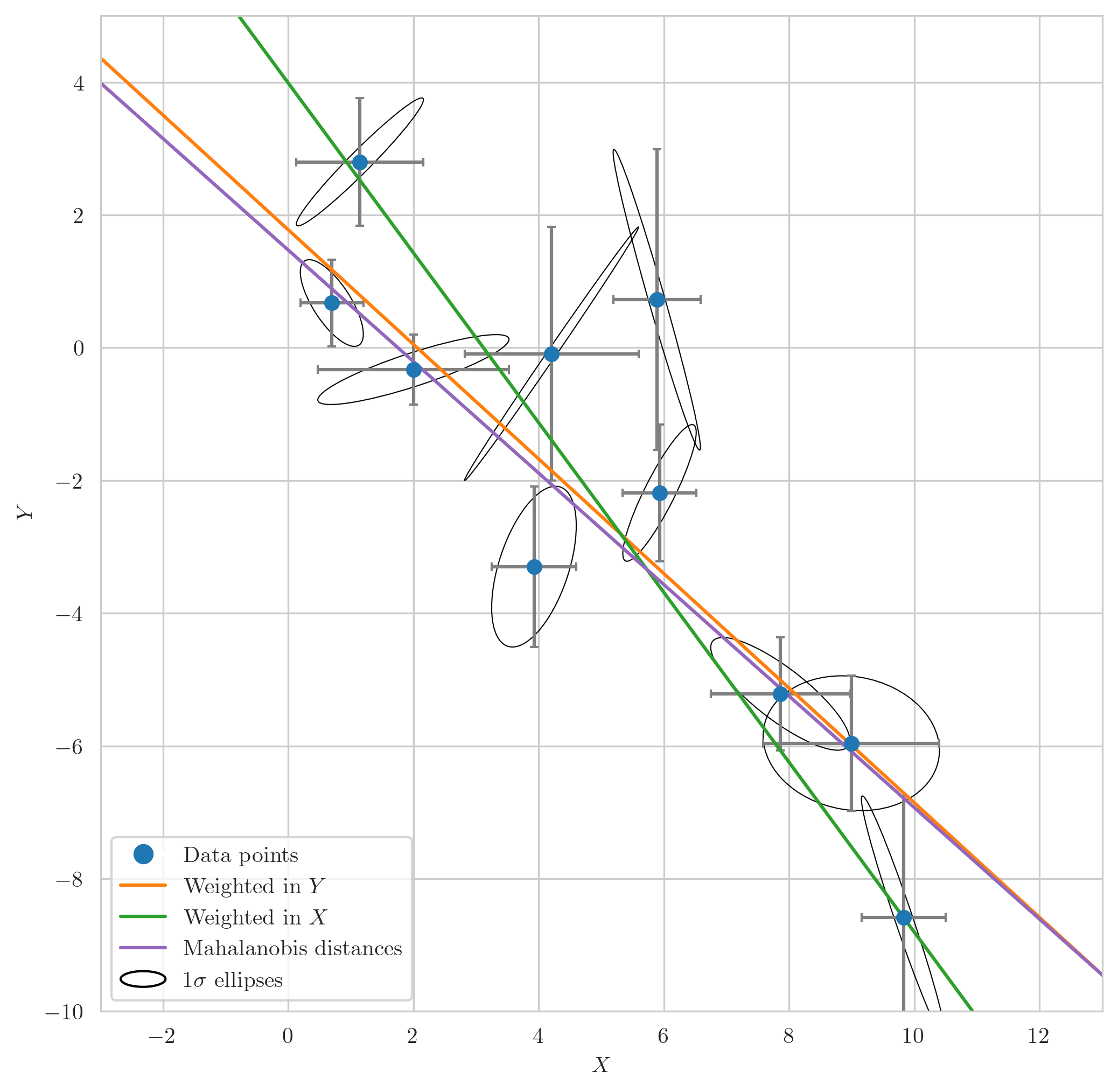 Visual representation of different methods to account for errors in a linear model fit. The orange line indicates a fit considering errors only in the y-direction. The green line corresponds to a fit considering errors in the x-direction. The purple line denotes the fit using Mahalanobis distance, which accounts for errors in both directions. Error bars and 1-sigma error ellipses around each data point visually represent measurement uncertainty and correlation.