Thoughts about Lasso Regression

I’ve been thinking about Lasso regression lately, and more specifically, about regularization. I wanted to see if there was a way to reformulate Lasso regularization as a quadratic convex problem. The answer seems to be, ‘yes, but at what cost?’ (pun only intended in hindsight).

A Simple Observation

I’ve never been fond of the absolute value function. I prefer thinking about it as $\vert w\vert=\sqrt{w^2}$. This transformation made me wonder, can we write a function that minimizes at $\sqrt{w^2}$? There are many possibilities, but today, let’s focus on this:

\[\Lambda(s,w)=\frac{1}{2}\left(s w^2+\frac{1}{s}\right).\]

Given that the domain is restricted to $s>0$, we have $\min_{s>0}\Lambda=\vert w\vert$. Why is this interesting? Because it’s a quadratic function in $w$. So, what does this have to do with Lasso regression?

Recall that in Lasso regression, we add the $L_1$ norm of the weights to the loss function. Specifically, if the unregulated loss function is $\ell(w)$, then the Lasso loss function is

\[\ell_{\rm lasso}(\boldsymbol{w})=\ell(\boldsymbol{w})+\lambda\Vert \boldsymbol{w}\Vert_1=\ell(\boldsymbol{w})+\sum_i\lambda\vert w_i\vert.\]

Our brief discussion about the $\Lambda$ function leads us to understand that the Lasso regression can also be written as

\[\ell_{\rm lasso}(\boldsymbol{w},\boldsymbol{s})=\ell(\boldsymbol{w})+\frac{\lambda}{2}\left[\boldsymbol{w}^T{\rm diag}[\boldsymbol{s}]\boldsymbol{w}+\sum_{i}s_i^{-1}\right],\]

where $\boldsymbol{s}$ is a vector of Lagrange multipliers, of the same dimension as $\boldsymbol{w}$. Effectively, we have doubled the weight space. So, what’s the benefit? The dependence on $\boldsymbol{w}$ is now quadratic, and the gradients with respect to both $\boldsymbol{w}$ and $\boldsymbol{s}$ are straightforward.

\[\boldsymbol{\nabla}_{\boldsymbol{w}}\ell_{\rm lasso}=\boldsymbol{\nabla}_{\boldsymbol{w}}\ell+\lambda\,{\rm diag}[\boldsymbol{s}]\boldsymbol{w}\;\;,\;\;\frac{\partial\ell_{\rm lasso}}{\partial s_i}=w_i^2-s_i^{-2}\]

Keeping in mind that $s_i>0$, it is also clear that $\ell_{\rm lasso}$ is convex, given that $\ell$ is. Note that to circumvent the $s>0$ restriction, we may define $s=e^\sigma$. Minimizing $\ell_{\rm lasso}(\boldsymbol{w},\exp\boldsymbol{\sigma})$ with respect to $\boldsymbol{\sigma}$ over the reals will also give the desired $L_1$ regulator.

The Simplest Example Possible - 1D Linear Regression

To illustrate what we might achieve with this new perspective, let’s consider a 1D linear Lasso regression, where our model has only one parameter, say $y=w x$. The loss function would be

\[\ell=\frac{1}{2}\Vert w\boldsymbol{x}-\boldsymbol{y}\Vert_2+\frac{\lambda}{2s}(s^2w^2+1).\]

The derivatives for $w$ is given by

\[\frac{\partial \ell}{\partial w}=w(x^2+\lambda s)-\boldsymbol{x}\cdot\boldsymbol{y}\;\;\Rightarrow\;\;w=\frac{\boldsymbol{x}\cdot\boldsymbol{y}}{x^2+\lambda s}.\]

Given that both $s$ and $\lambda$ are positive, we see that the regularization pushes the weights towards smaller values. Now, moving to the $s$ equation,

\[\frac{\partial \ell}{\partial s}=\frac{\lambda}{2}(w^2-s^{-2})\;\;\Rightarrow\;\;s^2=w^{-2}=\frac{(x^2+\lambda s)^2}{(\boldsymbol{x}\cdot\boldsymbol{y})^2}.\]

We can combine the two equations above into a single equation for $w$,

\[\boxed{w=\frac{\boldsymbol{x}\cdot\boldsymbol{y}}{x^2+\lambda\vert w\vert^{-1}}}.\]

Instead of solving this equation directly, I suggest viewing this as an iterative process. This implies the existence of a sequence of $w$ values, $w^{(i)}$, $i=1,2,…$ such that

\[w^{(i+1)}=\frac{\boldsymbol{x}\cdot\boldsymbol{y}}{x^2+\lambda\vert w^{(i)}\vert^{-1}}.\]

The convexity of the loss function assures the convergence of this process. By further setting $w^{(0)}=1$, the first iteration ($w^{(1)}$) gives the Ridge regression result. This insight allows us to interpret Lasso regression as a sequence of modified Ridge regression problems, as we next study in more depth.

Lasso Regression as a Sequence of Ridge regression Problems

Building on the simplified discussion above, I propose treating Lasso regression as a sequence of modified Ridge regression problems, expressed as

\[\ell^{(i)}\left(\boldsymbol{w},\boldsymbol{w}^{(i-1)}\right)=\ell(\boldsymbol{w})+\frac{\lambda}{2}\boldsymbol{w}^TD[\boldsymbol{w}^{(i-1)}]\boldsymbol{w}\;\;,\;\;D[\boldsymbol{w}]={\rm diag}\left[\vert w_1\vert^{-1} ,\vert w_2\vert^{-1} ,...,\vert w_N\vert^{-1} \right]\]

with $\boldsymbol{w}^{(0)}=\mathbb{1}$, and $\boldsymbol{w}^{(i>0)}$ are the weights minimizing $\ell^{(i)}$. Repeating this iteratively, will eventually converge to the same minimum as the Lasso regression.

The Next Simplest Example Possible - linear regression

To further illustrate this approach, let’s examine a regularized linear regression problem. In this case, we have

\[\ell^{(i)}=\frac{1}{2N}\Vert X\boldsymbol{w}-\boldsymbol{y}\Vert_2+\frac{\lambda}{2}\boldsymbol{w}^TD^{(i-1)}\boldsymbol{w},\]

where $N$ is the number of samples. The normal equations are simply

\[\left(X^TX+\lambda ND^{(i-1)}\right)\boldsymbol{w}^{(i)}=X^T\boldsymbol{y}\;\;,\;\; D^{(0)}=\mathbb{I}.\]

In the near future, I will follow up on this post with a more detailed discussion of numerically implementing this method in some more sophisticated settings, where analytical solutions can’t get us far. But for the time being, to investigate this numerically, I have set up a simple Python experiment using the California Housing dataset from Scikit-learn. I applied the Lasso sequence Ridge function for a specific $\lambda$, and tracked the evolution of each weight over iterations. The full Python notebook is available on GitHub, but the code snippet below provides an overview of the method.

def lasso_sequence_ridge(X, y, lambda_, num_iterations):
    n_samples, N = X.shape  # the number of features and samples
    w = np.ones(N)  # initialize the weights
    w_history = []  # list to store the history of weights

    # scale the lambda by the number of samples
    lambda_scaled = lambda_  * n_samples
    for i in range(num_iterations):
        D = np.diag(1/np.abs(w))  # diagonal matrix of absolute weights
        # solve the normal equations
        w = np.linalg.inv(X.T @ X + lambda_scaled * D) @ X.T @ y
        w_history.append(w)

    return np.array(w_history)

Setting $\lambda=0.1$, we compared the obtained weights to those from the standard Lasso regression as implemented in scikit-learn. The weights from our sequence of Ridge regressions converged to values very similar to those from the Lasso regression, validating our approach.

from sklearn.linear_model import Lasso
lasso = Lasso(alpha=lambda_)
lasso.fit(X, y)

print("Final weights from Lasso:")
print([f'{x:.3f}' for x in lasso.coef_])
print("Final weights from sequence of Ridge regressions:")
print([f'{x:.3f}' for x in w_history[-1]])

The output is

Final weights from Lasso:
['0.706', '0.106', '-0.000', '-0.000', '-0.000', '-0.000', '-0.011', '-0.000']
Final weights from sequence of Ridge regressions:
['0.706', '0.106', '-0.000', '-0.000', '-0.000', '-0.000', '-0.013', '-0.000']

The plot below visualizes how each weight in the model evolves over the course of iterations, starting from the initial Ridge-like weights and converging towards their final values.

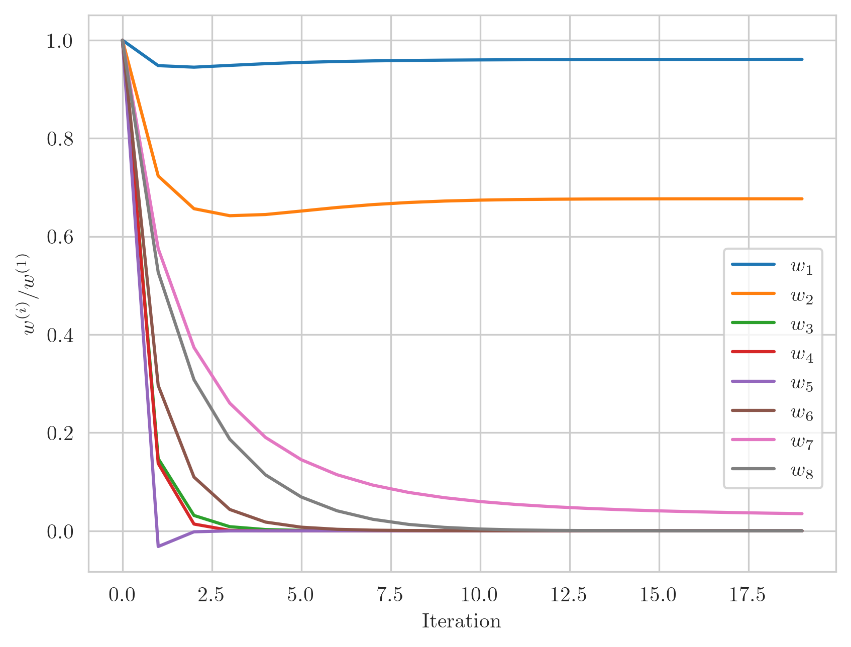Convergence of the weights in Lasso regression as a sequence of Ridge regression problems. Each curve represents the evolution of a single weight parameter normalized by its initial value. Notice how all curves eventually converge to their final values, demonstrating the process of gradual ‘feature selection’.