Interpretability project - nanoGPT trained on a WhatsApp group chat
A few months ago I decided to train Karpathy’s nonGPT on one of my WhatsApp group chats. This is a group of nine friends, and we have been chatting (quite intensively) for the past ten(!) years. What started as a joke, ended up being a very interesting project. Even though it is a character-level model, looking at the generated text, I realized that the model had learned a few interesting structural (and not so structural) patterns of our conversations. This post presents my attempts at understanding some things the model has learned, and how it learned them. A notebook including most of the calculations and visualizations can be found here.
The two main observations and an interpretation
- The model respects causality: Timestamps are generated in the correct order.
- The model distinguishes between group members: Some group members are ‘replied to faster’ than others.
Before I present the evidence for these observations, to keep the right context in mind, I want to describe my current understanding/interpretation of the mechanism the gives rise to these observations.
In the mechanistic interpretability literature, one important concept is the idea of ‘induction heads’. Very loosely, induction heads look for past occurrences of sequences ‘similar’ to the current sequence of tokens, and use them to predict the next token. Still very loosely, they are responsible for sequences of the form: [*A][*B]...[A]->[B], where *A is ‘similar’ to A under some metric, and *B is predicted such that it is similar to B under the same metric, while also being related to *A, in a similar sense to how B is related to A.
The way I currently understand the two observations above is very similar to the concept of induction heads. As we will see later in this post, I have identified 3 types of attention heads involved in the next-time-prediction task:
- Heads attending to the current ‘location’ in the previous timestamp (for instance, attending to minutes when predicting minutes).
- Heads attending to the next ‘location’ in the previous timestamp (for instance, attending to seconds when predicting minutes).
- Heads attending to the last sender.
I think that those three groups of heads are part of a circuit that produces sequences to the form:
[_begin_][hh][mm][ss][sender]...->[_begin_][*hh][*mm][*ss]...
where [_begin_] marks the beginning of a message, and *X is similar to X in some sense. The interesting part is that the predicted timestamp, [*hh][*mm][*ss], is always in the future of the previous one. Moreover, the second timestamp is predicted in a very structured way; for example, it seems as if the model predicts *mm=mm+d1(ss)+d2(sender), where d1 and d2 are some positive functions of the previous message seconds and sender, respectively. I’m tempted to guess that these are some type of ‘convolutional induction heads’, in the sense that the induction is ‘copying’ time differences rather than the actual time. I don’t have evidence for that claim yet, but would be interesting to explore this more systematically.
Below I present the evidence I have for these two observations.
Observation 1: Correct timestamps + sender structure
Let’s look at an example of a conversation generated by the model: (To protect privacy, the content of the messages and sender names have been erased, but the timestamps are kept).
1
2
3
4
5
6
7
[06/03/2021, 9:04:30] Member 2: [message 1, erased for privacy]
[06/03/2021, 9:04:40] Member 2: [message 2, erased for privacy]
[06/03/2021, 9:04:53] Member 9: [message 3, erased for privacy]
[06/03/2021, 9:10:38] Member 6: [message 4, erased for privacy]
[06/03/2021, 9:10:58] Member 2: [message 5, erased for privacy]
[06/03/2021, 9:11:04] Member 4: [message 6, erased for privacy]
...
The first thing that caught my eye was the correct structure of the timestamps and the sender names. Recall that this is a character-level model, so I was quite pleased to see that it had learned the structure of the timestamps and the sender names. In all my experiments, the model never generated a timestamp that was not in the correct format and the correct order, meaning, the timestamps are always increasing.
Later in this post, I will claim that the model also learned to distinguish between the different senders. For that reason, I re-trained the model with each sender’s name represented by a dedicated token, other than that, the model was trained on single characters. For consistency, throughout this post I will always use the model trained with the tokenized sender names.
Context length:
For the model to be able to learn the increasing nature of the timestamps, it must have a context long enough to contain at least two consecutive timestamps. Below is a histogram of message lengths in the training data, which shows that the model context size of 256 is enough to contain many instances of more than a single timestamp.
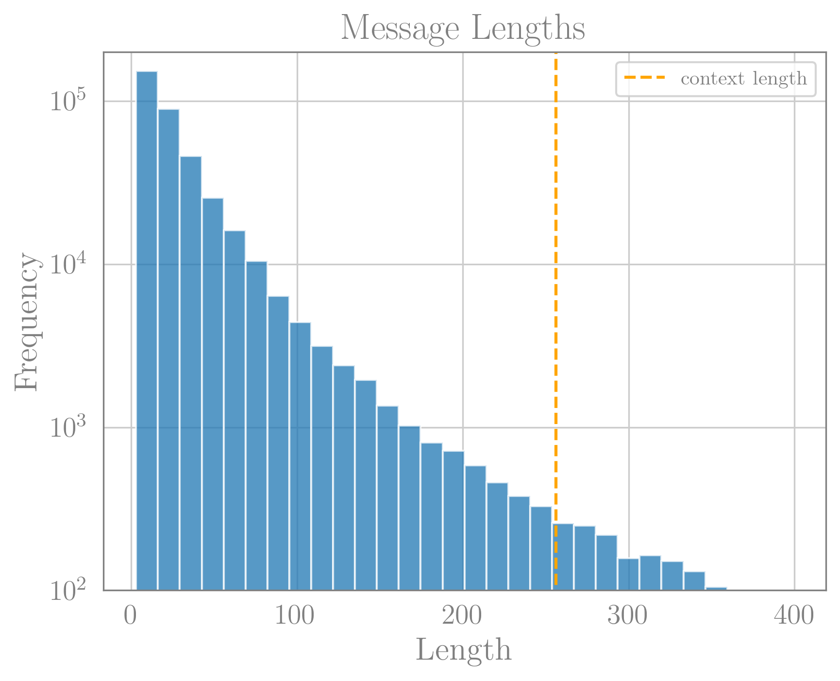 Distribution of massage lengths in the training data. Orange line represents the model context size of 256. We see that there are many messages much shorter than 256.
The model learned causality:
Next, I went on to try a time prediction task. I prompted the model with a timestamp and a fake message:
prompt = '[04/11/2022, 18:29:50] Member 2: Some text.\n[04/11/2022, 18:'
The probabilities for the next character are given below:
| Next Token | Probability |
|---|---|
| 3 | 67.87% |
| 2 | 23.38% |
| 4 | 6.69% |
| 5 | 1.85% |
| 1 | 0.11% |
| 0 | 0.09% |
We see that the model gives a very low probability to the next character being in the past, namely, being 0 or 1. This is a very interesting result, as it shows that the model has learned that time stamps should only increase. It also seems like the model learned that 3 is more likely to be the next character than 2. This is very reasonable, since there is only a short amount of time after 18:29:50 that a timestamp of the form 18:2x:xx makes sense.
To be clear, the above is just a single example, but I have prompted the model with multiple timestamps and messages, and the model always gave very low probabilities for past timestamps.
Induction heads?
To try and get a better understanding of how the model actually predicts the next character, I studied the attention weights of the model. I was hoping to see that the model attends to the previous timestamp when predicting the next one, like attention heads do. I did find seven heads in the model that attend to the previous timestamp when predicted the next, all of them are in the 4th to 6th attention layers. The table below illustrates the attention mechanism of a specific head in the model as it processes a sequence. Each row shows the attention distribution over past tokens. The box on the right in each row marks the ‘current’ token. The green shadings indicate the strength of the attention on each token. The numbers in parentheses represent the zero-indexed (layer, head) shown.
I have also identified one special head, that appear to attend to the ‘next number of the previous timestamp’. For example, if the previous timestamp was 7:23:45, the model would attend to the 4 when predicting the minutes of the next timestamp. This head is the (4,3) head, and it is shown below:
| [ | 0 | 4 | / | 1 | 1 | / | 2 | 0 | 2 | 3 | , | 1 | 8 | : | 2 | 2 | : | 2 | 1 | ] Member 1: | r | a | n | d | o | m | t | e | x | t | . | [ | 0 | 4 | / | 1 | 1 | / | 2 | 0 | 2 | ||||||||||
| [ | 0 | 4 | / | 1 | 1 | / | 2 | 0 | 2 | 3 | , | 1 | 8 | : | 2 | 2 | : | 2 | 1 | ] Member 1: | r | a | n | d | o | m | t | e | x | t | . | [ | 0 | 4 | / | 1 | 1 | / | 2 | 0 | 2 | 3 | |||||||||
| [ | 0 | 4 | / | 1 | 1 | / | 2 | 0 | 2 | 3 | , | 1 | 8 | : | 2 | 2 | : | 2 | 1 | ] Member 1: | r | a | n | d | o | m | t | e | x | t | . | [ | 0 | 4 | / | 1 | 1 | / | 2 | 0 | 2 | 3 | , | ||||||||
| [ | 0 | 4 | / | 1 | 1 | / | 2 | 0 | 2 | 3 | , | 1 | 8 | : | 2 | 2 | : | 2 | 1 | ] Member 1: | r | a | n | d | o | m | t | e | x | t | . | [ | 0 | 4 | / | 1 | 1 | / | 2 | 0 | 2 | 3 | , | ||||||||
| [ | 0 | 4 | / | 1 | 1 | / | 2 | 0 | 2 | 3 | , | 1 | 8 | : | 2 | 2 | : | 2 | 1 | ] Member 1: | r | a | n | d | o | m | t | e | x | t | . | [ | 0 | 4 | / | 1 | 1 | / | 2 | 0 | 2 | 3 | , | 1 | |||||||
| [ | 0 | 4 | / | 1 | 1 | / | 2 | 0 | 2 | 3 | , | 1 | 8 | : | 2 | 2 | : | 2 | 1 | ] Member 1: | r | a | n | d | o | m | t | e | x | t | . | [ | 0 | 4 | / | 1 | 1 | / | 2 | 0 | 2 | 3 | , | 1 | 8 | ||||||
| [ | 0 | 4 | / | 1 | 1 | / | 2 | 0 | 2 | 3 | , | 1 | 8 | : | 2 | 2 | : | 2 | 1 | ] Member 1: | r | a | n | d | o | m | t | e | x | t | . | [ | 0 | 4 | / | 1 | 1 | / | 2 | 0 | 2 | 3 | , | 1 | 8 | : | |||||
| [ | 0 | 4 | / | 1 | 1 | / | 2 | 0 | 2 | 3 | , | 1 | 8 | : | 2 | 2 | : | 2 | 1 | ] Member 1: | r | a | n | d | o | m | t | e | x | t | . | [ | 0 | 4 | / | 1 | 1 | / | 2 | 0 | 2 | 3 | , | 1 | 8 | : | 2 |
It is clearly seen that the attention in this head is shifted by one to the right relative to the previous examples.
I find the heads attending to the same number in the previous timestamp quite in-line with the concept of induction heads, as they seem to be learning a pattern in the data: previous timestamp -> next timestamp. However, the head that attends to the ‘next number of the previous timestamp’ appears to be more nuanced. As I discussed in the introduction, I think this head is part of a circuit that predicts the next timestamp by ‘copying’ time differences, rather than the actual time.
Observation 2: Different response times for different members
The second observation I made was that the model seems to ‘reply’ to some members faster than others. To test this, I prompted the model with a fixed arbitrary message and timestamp, changing only the sender. The prompt was in the following text:
'[04/11/2023, 18:21:13'+member_token+'Yesterday I woke up sucking a lemon.\n[04/11/2023, 18:':
Meaning, the model output for this prompt should be the first minute token of the next timestamp. The table below shows the top 2 predictions for the next token, for each member:
| Member | Prob. Next Token = 2 | Prob. Next Token = 3 |
|---|---|---|
| 1 | 88.46% | 6.19% |
| 2 | 89.13% | 5.84% |
| 3 | 89.58% | 5.58% |
| 4 | 90.19% | 5.33% |
| 5 | 89.21% | 5.75% |
| 6 | 92.37% | 4.23% |
| 7 | 88.83% | 5.92% |
| 8 | 88.08% | 6.33% |
| 9 | 88.73% | 6.06% |
It seems like the model has learned that member 6 likely to receive a reply faster than the other members. If this is indeed the case, we expect to see that the model ‘attends’ to the previous sender when predicting the next timestamp. In this case I have identified three heads that seem to attend to the previous sender when predicting the next timestamp. Bellow is the attention distribution for those heads, each line this time is for a different sender. Again the ‘buttons’ below represents the (layer, head) of the attention head shown.
It certainly seems like the model is attending to the previous sender when predicting the next timestamp. Specifically, the (3,3) head seems to attend to Member 6 more than it does to the other members. This is in line with the observation that the model ‘replies’ to Member 6 faster than to the other members.
Closing remarks and future directions
The two observations I presented here are quite intriguing to me. The evidence I have presented, however, are somewhat circumstantial. Moreover, I’ve made a conjecture that the model ‘copies’ time differences rather than the actual time, but I don’t have any evidence for that claim. Accordingly, I think there are a few interesting directions that I should explore in the future:
- Time differences: I should systematically study the time differences between consecutive timestamps the model predicts. It would be interesting to see if the model indeed ‘copies’ time difference between the timestamps.
- Turn off features/heads: One way to test whether the heads I identified are indeed responsible for the observations I made, is to turn them off and see if the model stops respecting causality or stops distinguishing between the senders. In such small models, however, I’m afraid that turning off an entire head might have effects on the model’s performance that extend beyond the specific behavior I’m interested in.
One other direction I’m interested in exploring is the effect of sparsity on interpretability. I have trained quite a few of these nanoGPT models with our sparsity inducing optimization (see $p$WD paper and PAdam blog post). It would be interesting to see if those induction heads are still easily interpretable when the model is sparse.
I might update this post in the future with the results of any future experiments I conduct. In the meantime, I’m quite pleased with the amount of structure the model has learned, and what I was able to learn from it.