Generalization Toy Models - II
A second post about generalization toy models. In this post I aim to study the effect of sparsity inducing regularization schemes on generalization.
Logic and challenges
The first post focused on purely analytical results in linear models and demonstrated how and why ridge regularization can improve the ability of a model to generalize. In this post, I will focus on slightly more complex networks, demonstrating how sparsity inducing norms (specifically $L_1$ norm) can sometimes result in better generalization abilities.
The main idea is that often times when we train a model all the model weights converge to some finite values. However, the loss space might exhibit a continuum of global minima, along which the loss is constant. This suggests that our model is over-parametrized, albeit probably in some very non-trivial way. By sending some of the network’s weights to 0, sparsity inducing regularization acts against over parametrization. I don’t yet posses a satisfying argument as for how sparsity inducing may affect generalization, however, a ‘hand-waving’ argument might be that a sparser network is ‘simpler’ in the information-theoretical sense, and therefore tend to generalize better. It will be interesting to try and understand this better in the future from the leans of singular learning theory (see this great blog post by Jesse Hoogland).
In all the following examples I will compare the validation loss obtained in the unregulated case, to the one obtained with $L_2$ and $L_1$ regularization. The examples we are going to study are
- Sparse linear teacher-student model: This basically models what happens if we use irrelevant features in under-determined linear regression.
Over-parametrized two layers teacher-student model: Here we basically demonstrate what happens when we use an over-complicated network for an underlying linear model.
- Over-parametrized non-linear teacher-student model: This is the most important example, as it shows how sparsity inducing norms dynamically lead to simpler networks that generalize better.
The first step however, will be to introduce how are we going to implement $L_1$ norm in PyTorch. A notebook for reproducing all our results can be found on GitHub.
Gradient decent with $L_1$ regularization.
The $L_1$ norm (the absolute value function) is singular around 0, this is known to lead to somewhat unstable gradient decent. To bypass this, we will make use of proximal gradient methods, as described in this Wikipedia page. Without getting in to too many details, it can be shown that if $\boldsymbol{w}^*$ is the weight vector that minimizes $\ell(\boldsymbol{w})=\ell_0(\boldsymbol{w})+\lambda\Vert \boldsymbol{w}\Vert_1$, it is also the solution to the equation
\[\boldsymbol{w}^*=S_{\lambda\eta}\left[\boldsymbol{w}^*-\eta\boldsymbol{\nabla}_{\boldsymbol{w}^*}\ell_0(\boldsymbol{w}^*)\right],\]for any value of $\eta$, and where $S_{\lambda}$ is the soft thresholding operator
\[S_\lambda(x)={\rm sign}(x){\rm ReLU}({\rm abs}[x]-\lambda).\]To incorporate it into any PyTorch optimizer, we can simply add a soft thresholding step after the gradient update step, namely, we identify $\eta$ above as our learning rate, and update like so
\[\boldsymbol{w}\leftarrow \boldsymbol{w}-\eta\boldsymbol{\nabla}_{\boldsymbol{w}}\ell_0(\boldsymbol{w})\] \[\boldsymbol{w}\leftarrow S_{\eta \lambda}(\boldsymbol{w})\]In PyTorch, using torch.optim.SGD as an example, this is done like so:
1
2
3
4
5
6
7
8
9
10
11
12
13
14
15
16
17
18
class SGD_L1(torch.optim.SGD):
    def __init__(self, params, l1_lambda=0.01, *args, **kwargs):
        super(SGD_L1, self).__init__(params, *args, **kwargs)
        self.l1_lambda = l1_lambda

    @torch.no_grad()
    def step(self, closure=None):
        # standard SGD step
        loss = super(SGD_L1, self).step(closure)

        # Soft thresholding
        for group in self.param_groups:
            lr = group['lr']
            for p in group['params']:
                p.data = torch.sign(p.data) * torch.clamp(torch.abs(p.data) - self.l1_lambda * lr, min=0)

        return loss
For the case of SGD, rewriting the whole optimizer would be rather simple, however the nice thing about the above method is that it can be applied to whichever optimizer we want.
Toy Examples
First example: sparse linear regression.
The setup here is almost identical to the one used in the previous post. We have a set of $N_{\rm tr}$ training samples, each is vector $\boldsymbol{X}$ in ${\mathbb{R}}^D$, where $N_{\rm tr}\lesssim D$. $\boldsymbol{X}$ is drawn from a standard normal distribution, so that design matrix $X\in\mathbb{R}^{D\times N_{\rm tr}}$ is a matrix of ${N_{\rm tr}\times D}$ iid standard normal random variables. $\boldsymbol{S},\boldsymbol{T}\in\mathbb{R}^D$ are the student and teacher vectors respectively. The Gram matrix for our data set is given by $\Sigma_{\rm tr}=XX^T/N_{\rm tr}$, and its population mean is simply given by a $D\times D$ identity matrix. We assume an MSE loss function $(\boldsymbol{S}-\boldsymbol{T})^T\Sigma_{\rm tr}(\boldsymbol{S}-\boldsymbol{T})/2$ for training, and test for generalization by taking the population mean of the loss, $\Vert \boldsymbol{S}-\boldsymbol{T} \Vert_2^2/2$.
We will use normalized teacher vectors, $\Vert\boldsymbol{T} \Vert_2^2=1$ and train the student vector, first by choosing a random unit teacher vector in $\mathbb{R}^D$, and then by choosing a unit vector in $\mathbb{R}^{d}{\subset}{\mathbb{R}}^D$, and padding it by $D-d$ zeros. The second case is similar to assuming that only $d$ out of the $D$ features we use actually effect our loss. We train the student using three different optimizers; unregularized, ridge, and lasso. Since the unregularized loss and ridge loss are invariant under orthogonal transformation of the student vector (“Spherical symmetry”), we don’t expect to see any difference in the ability of the model to generalize regardless of the subspace from which $\boldsymbol{T}$ is selected. We therefore expect that the generalization loss in those cases will be given by the results in the previous post:
\[\ell_{\mathrm{gen},0}\simeq\frac{1}{2}\left(1-\frac{N_{\rm tr}}{D}\right)\Vert \boldsymbol{S}_0-\boldsymbol{T}\Vert_2^2\;\;,\;\;\ell_{\mathrm{gen},L_2}\simeq\frac{1}{2}\left(1-\frac{N_{\rm tr}}{D}\right)\Vert \boldsymbol{T}\Vert_2^2+{\cal O}(\lambda^2)\]The $L_1$ norm, however, does depend on the basis of $\mathbb{R}^D$ we work in. For that reason, together with the fact that it induces sparsity, we expect it to outperform in the sparse case.
Below we show a plot demonstrating precisely these observations; the generalization in the unregularized and ridge case practically aren’t affected by the direction of $\boldsymbol{T}$. The lasso case on the other hand preforms much better than others for sparse teacher. For a random teacher however, ridge outperforms lasso. The parameters used for these plots are $D=1000,\;N_{\rm tr}=700$, and in the sparse case we set $d=400$. For the hyperparameters (learning rate and weight decay) in the unregularized and ridge cases we used the optimal parameters as described in the previous post. For the lasso case we used $\eta=0.4$ and $\lambda=5\times10^{-3}$, without trying too hard to optimize.
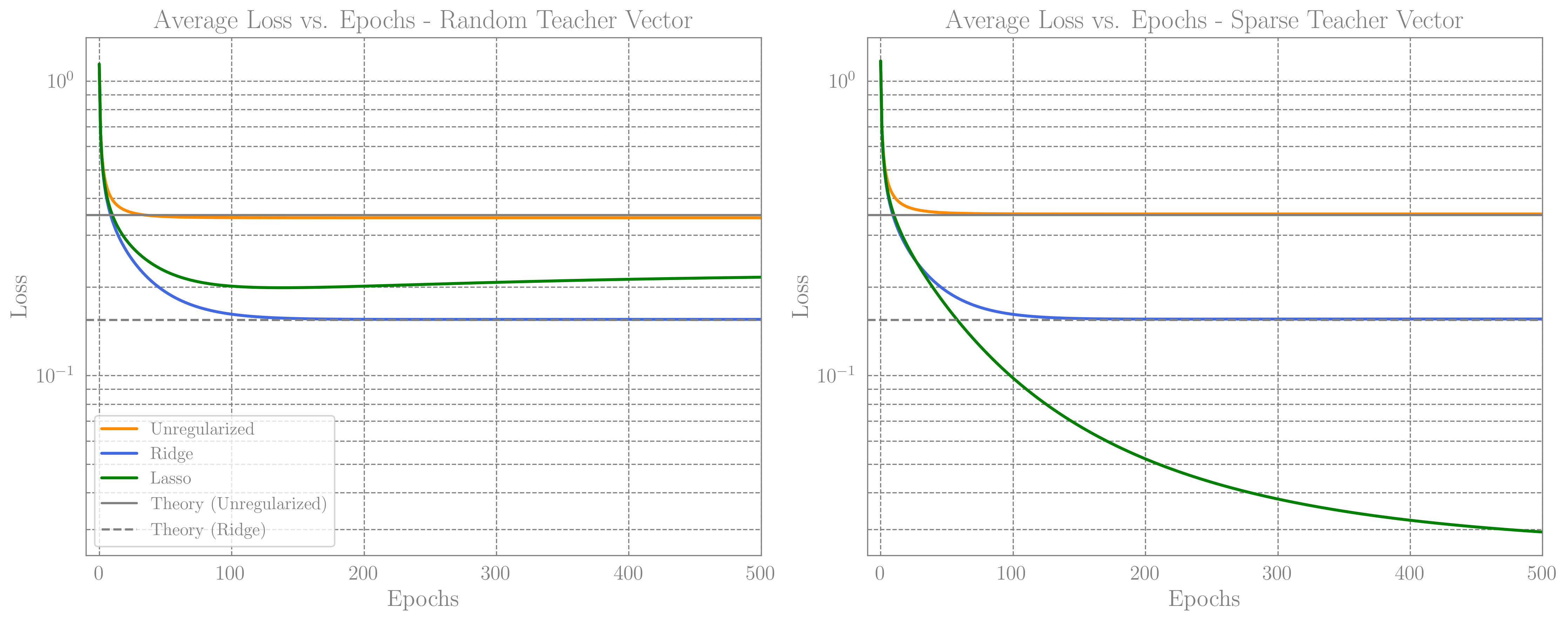 Average loss curves vs epochs, for a random teacher vector and a $70\%$ sparse vector. We see that while for a random teacher Ridge outperforms Lasso, Lasso generalizes much better in the case of Sparse network.
I’m unable to “prove” this, but my intuition is that the $L_1$ norm basically reduces the effective dimension from $D$ to $d$. Therefore, in the case we consider, where $d<N_{\rm tr}$, we can expect that the data we have is sufficient to learn the $d$ non-vanishing entries of $\boldsymbol{T}$.
An over parametrized linear model, diguised as a non-linear model
To elaborate on the intuition above a bit further, I think that the important thing here is that in the sparse $\boldsymbol{T}$ example, there are indeed only $d$ features that play a role. As a counter example, consider the case where we over-parametrize the model by adding a linear layer, such that now $\boldsymbol{S}=M\boldsymbol{V}$, for some matrix $M \in \mathbb{R}^{D\times m}$ and $\boldsymbol{V}\in\mathbb{R}^{m}$, while $\boldsymbol{T}$ is still some arbitrary unit vector. In this realization, there are infinity many pairs of $M$ and $\boldsymbol{V}$ giving the same $\boldsymbol{S}$. The $L_1$ regularization, if applied correctly, will probably find a specific configuration where $\boldsymbol{V}$ has only a single non-vanishing entry, and $M$ has only a single non-vanishing column. But from the point of view of the entire network, the only thing that effects the ability of the model to generalize, (or any other preference matrix), is the resulting vector $\boldsymbol{S}$. Below is a matrix plot of the weights $M$, in the case where $D=400,\;m=600$. As is clearly seen, only three columns of $M$ are actually used in the lasso trained network, while in the ridge case far less structure is observed. The performance of both networks is basically identical and comparable to the theatrical predictions of the linear case.
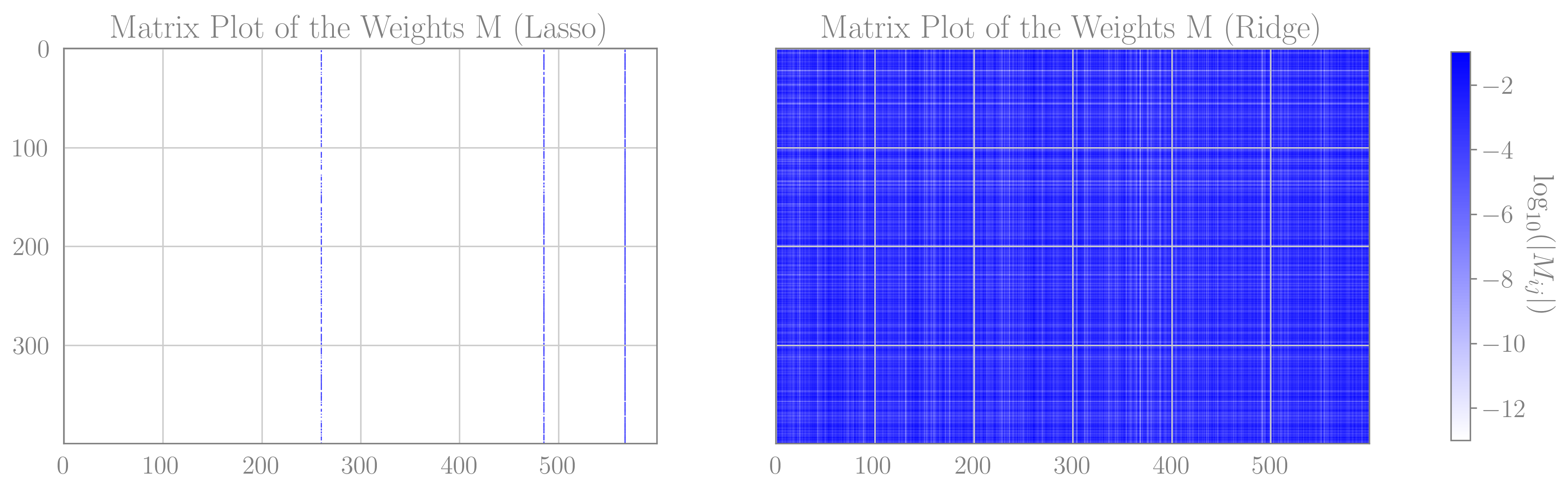 Matrix plots for the absolute value of the weights in an $L_1$ regularized network (left) and $L_2$ regularized network (right)
An over-parametrized non-linear model
So far in the last two posts, I’ve looked only at effectively linear models, where the teacher and student vectors are linear functions of the data. In this example I’m going to consider a non-linear model with a single hidden layer followed by a ReLU activation function. The data would still be Gaussian, but the dimension will be smaller $D=100$, the hidden layer in the teacher network will have a size of 10, and the “over-parametrized” student network will have a hidden layer of size 100. We will again assume an “under-constrained” scenario, where we have only 60 (<100) samples drawn randomally.
After quite a few attempts to optimize both the networks with both $L_2$ and $L_1$ regularization, It does seem that the $L_1$ optimizer obtained negligibly better generalization loss. The $L_1$ optimizer did, however, set about $89\%$ of the weights in the hidden layer to zero, nearly matching the teacher net, which had a hidden layer of size 10 instead of a 100. The $L_2$ optimizer, on the other hand, did not seem to prefer a smaller hidden layer dimension, as expected.
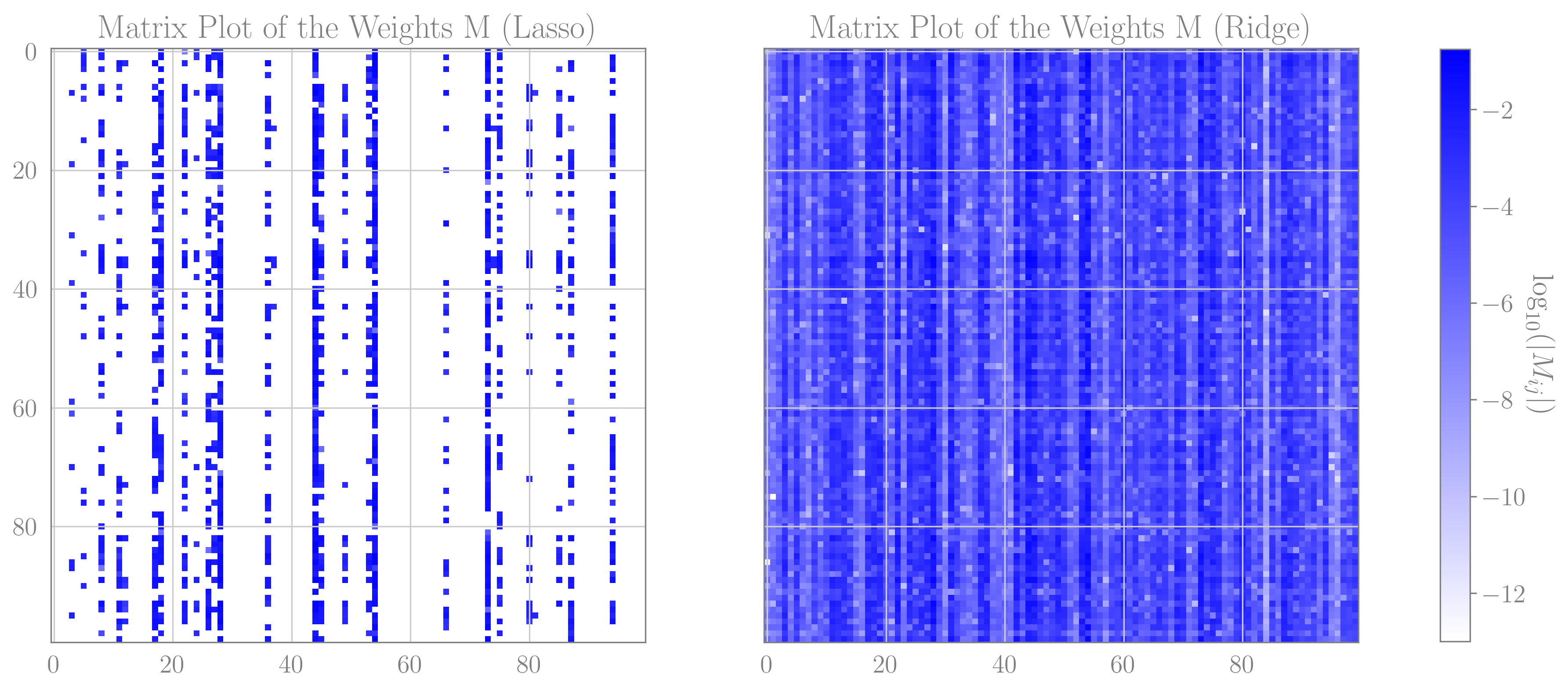 Matrix plots for the absolute value of the weights in an $L_1$ regularized network (left) and $L_2$ regularized network (right), for a model with a nonlinear hidden layer
The ability to generalize and the relation to sparsity in realistic settings is still unclear to me. I would want to re-visit this in the near future, my first guess would be to try and understand it from the singular learning theory point of view.