Generalization Toy Models - I
As part of my attempts at better understanding Lasso regularization (more on that to come soon!), I’ve been thinking more broadly about regularization in ML recently. One thing I was able to understand slightly better, is the ability of certain regularization schemes to increase the ability of a model to generalize. In the two following blog posts, I’m going to discuss those findings, mainly in the context of a very simple teacher-student model. This first blog post will be strictly devoted to analytical results, while the subsequent one is going to focus on numerical aspects of more involved toy models.
Logic
There are two main points I want to make in the next two blog posts:
- Given a set of training data, it is possible that some direction in model parameters space will have no effect the model loss. This is generally true when the number of data examples is smaller than its dimension. We will refer to such directions as ‘flat-directions’. Adding a regularization term tend to ‘lift’ those flat directions, usually in a way that acts to set such ‘flat-parameters’ to zero. This effect tends to improve the model ability to generalize, and reduces the dependence on initialization.
- An over-parameterized network usually exhibit many flat-directions. In such cases lasso (or any $L_p$ with $p<1$) regularization tend to result in very sparse network, which generally improve generalization.
The first point is covered in this post, while the second will be discussed in the next post.
Toy Model Calculations
In this post, I will focus on a very simple teacher-student model. I will assume my data is a set of $N_{\rm tr}$ training examples, each of which is a vector $\boldsymbol{X}$ of length $D$, such that $N_{\rm tr}\lesssim D$. I will further assume that each vector $\boldsymbol{X}$ is drawn from a standard normal distribution, the design matrix $X\in\mathbb{R}^{D\times N_{\rm tr}}$ is therefore essentially a collection of ${N_{\rm tr}\times D}$ iid standard normal random variables. The Gram matrix for this data set is given by $\Sigma_{\rm tr}=XX^T/N_{\rm tr}$, and its population mean is simply given by a $D\times D$ identity matrix. The first two examples we are going to study are strictly linear. $\boldsymbol{S},\boldsymbol{T}\in\mathbb{R}^D$ are the student and teacher vectors respectively, and the difference between them is denoted by $\boldsymbol{D}=\boldsymbol{S}-\boldsymbol{T}$. The MSE loss and its gradient are given by
\[\ell_{\rm tr}=\frac{1}{2}\boldsymbol{D}^T\Sigma_{\rm tr}\boldsymbol{D}\;\;\Rightarrow\;\;\frac{\partial \ell_{\rm tr}}{\partial \boldsymbol{S}}=\frac{\partial \ell_{\rm tr}}{\partial \boldsymbol{D}}=\Sigma_{\rm tr}\boldsymbol{D}.\]Since the average over all possible data sets of $\Sigma_{\rm tr}$ is $\left\langle\Sigma_{\rm tr}\right\rangle_X=I$, when we test how well this model generalizes, we will assume the population mean of the above loss, $\ell_{\rm gen}=\boldsymbol{D}^T\boldsymbol{D}/2$. For the time being, we care mainly about the steady state of the system, the dynamics will be studied with some more details towards the end of this post. For that reason, we will currently work in the gradient flow limit.
Unregularized case
In this case the weights evolve according to
\[\dot{\boldsymbol{D}}=\dot{\boldsymbol{S}}=-\Sigma_{\rm tr}\boldsymbol{D}\;\;,\;\;\boldsymbol{S}(0)=\boldsymbol{S}_0.\]This solution to this equation can be expressed formally with matrix exponentiation, however, we find it more instructive to move to the (orthonormal) eigen-basis of $\Sigma_{\rm tr}$
\[\Sigma_{\rm tr} \boldsymbol{v}_i=\lambda_i\boldsymbol{v}_i\;\;,\;\;\boldsymbol{v}_i^T\boldsymbol{v}_j=\delta_{ij},\]where $\lambda_i$ are the eigenvalues of $\Sigma_{\rm tr}$ and $\delta_{ij}$ is the Kronecker delta. Writing $S$, $T$, and $D$ in this basis, we get that each component evolves independently of the others, giving
\[S_{i}(t)=T_i+(S_{i,0}-T_i)e^{-\lambda_i t}.\]The generalization loss as a function of time in that case is thus simply given by
\[\ell_{\rm gen}=\frac{1}{2}\sum_{i=1}^D(S_{i,0}-T_i)^2e^{-2\lambda_i t}.\]We recall that $\Sigma_{\rm tr}$ is the Gram matrix of $N_{\rm tr}$ samples of $D$-vectors. Its eigenvalues are therefore non-negative. Moreover, since we focus on $N_{\rm tr}<D$, it has at least $D-N_{\rm tr}$ vanishing eigenvalues. As $t\to\infty$, the contribution of all eigenvectors associated with positive eigenvalues to the loss will decay exponentially. Vectors in the null-space of $\Sigma_{\rm tr}$ will not evolve, this is the space of ‘flat-directions’. The population average (average over all possible data-sets) of the generalization loss above can be evaluated analytically in some limiting cases using the Marchenko-Pastur theorem. However, since our data is drowned from an isotropic distribution, each direction in $\mathbb{R}^D$ will have the same probability to be associated with a $0$ eigenvalue. We also know that on average there will be exactly $D-N_{\rm tr}$ vanishing eigenvalues. The population mean of the generalization loss is therefore given by
\[\lim_{t\to\infty}\left\langle\ell_{\rm gen}\right\rangle_{X}=\frac{1}{2}\left(1-\frac{N_{\rm tr}}{D}\right)\Vert \boldsymbol{S}_0-\boldsymbol{T}\Vert_2^2.\]It is common to initialize the student weights $\boldsymbol{S}_0$ by selecting it from a zero-mean distribution. In which case the mean expected loss will be given by
We see explicitly the sensitivity to weights initialization.
Ridge regularization
In the ridge case, we add the regularization term $\lambda\Vert \boldsymbol{S}\Vert_2^2$ to the loss $\ell_{\rm tr}$, the components of $S$ eigenbasis of $\Sigma_{\rm tr}$ evolve according to the following gradient flow
\[\dot{S}=-(\lambda_i+\lambda)S_i+\lambda_iT_i,\]which is solved by
\[S_i(t)=\left(S_{i,0}-\frac{\lambda_i}{\lambda+\lambda_i} T_i\right )e^{-(\lambda+\lambda)t}+\frac{\lambda_i}{\lambda+\lambda_i}T_i.\]At the $t\to\infty$ limit, the generalization loss will be given by
This expression can, too, be analytically estimated using the Marchenko-Pastur eigenvalues distribution. However, if we assume that $\lambda$ is small enough, we see, again, that only the $\lambda_i=0$ subspace contributes to the loss, resulting with a mean estimated loss of
This loss is generally lower than the one in unregularized case as given in Eq.[1], and independent of $S_0$. This is a demonstration of the first point we wanted to discuss, and gives a simplistic understanding as to how regularization can improve the ability of a model to generalize.
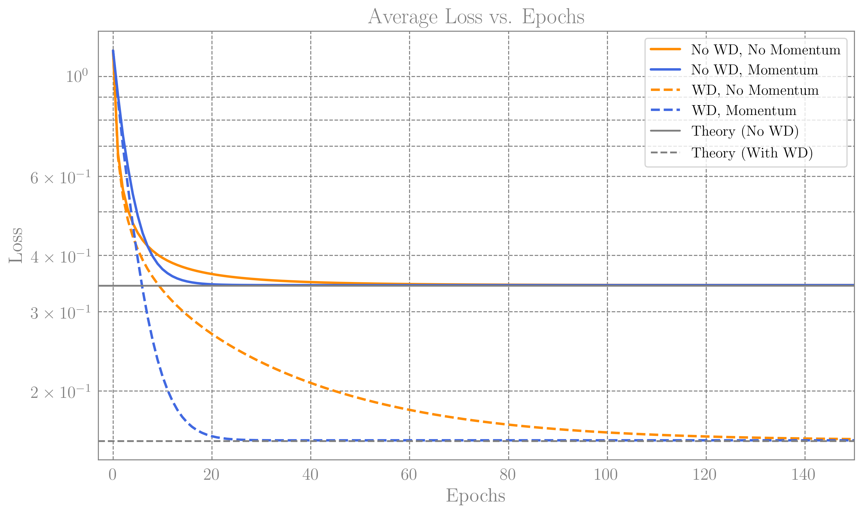 Average loss curves vs epochs. The plot was made for the case of $D=1000$, $N{\rm tr}=700$, and we averaged over 100 randomally generated data sets ($X$ and $\Sigma_{\rm tr}$). The selection of hyperparameters is discussed below. We see that the finite step size learning match the predictions of Eq.[1] and Eq.[3], where we included the finite $\lambda$ correction to Eq.[3]._
Numerics
To verify the above derivations, I’ve implemented our simple model in PyTorch. The notebook can be found on GitHub.
The numerical implementation obviously uses finite learning rates and step sizes, which I selected based on the wonderful discussion about Why Momentum Really Works in Distill.pub. The convergence rate of the training loss, sensitive to the largest and smallest (non-vanishing) eigenvalues of the Hessian, which in our case is either $\Sigma_{\rm tr}$ or $\Sigma_{\rm tr}+\lambda I$ in the ridge case. The vanishing eigenvalues are associated with flat directions that don’t learn, and therefore don’t affect the convergence rate. Following the Distill article, the optimal learning rate in our case will be given by
\[\eta_{0}=\frac{2}{\lambda_{+}+\lambda_{-}}\;\;,\;\;\eta_{\lambda}=\frac{2}{\lambda_{+}+2\lambda},\]where $\eta_0\,, \eta_{\lambda}$ are the learning rate in the unregualted and ridge cases respectively, and $\lambda_{\pm}$ are the largest and smallest eigenvalues of $\Sigma_{\rm tr}$. The corresponding optimal convergence rates are given by
\[R_0=\frac{\lambda_{\rm max}/\lambda_{\rm min}-1}{\lambda_{\rm max}/\lambda_{\rm min}+1}\;\;,\;\;R_{\lambda}=\frac{\lambda_{\rm max}/\lambda}{\lambda_{\rm max}/\lambda+2}\;.\]As seen from Eq.[2], the generalization loss is an increasing function of $\lambda$, which motivates using the smallest $\lambda$ possible. The convergence rate $R_\lambda$ above, however, shows that learning in the $\lambda\to 0$ limit will be very slow. To somewhat balance the two, we will choose $\lambda$ such that the learning rates are equal, $R_0=R_\lambda$, giving
\[\lambda_R=\frac{\lambda_+\lambda_-}{\lambda_+-\lambda_-}\]In the limit of $D\to\infty$ ad fixed $q=N_{\rm tr}/D$, $\lambda_{\pm}$ are given as part of the Marchenko-Pastur theorem by $\lambda_{\pm}=(1\pm\sqrt{D/N_{\rm tr}})^2$, the learning rates and $\lambda_R$ are then given by
\[\lambda_R=\frac{(1-q)^2}{4q^{3/2}}\;\;;\;\;\eta_0=\frac{q}{1+q}\;\;,\;\;\eta_{\lambda}=\frac{4q^{3/2}}{(1+q)(1+\sqrt{q})^2}.\]In the same limit, when setting $\lambda=\lambda_R$, it can be shown that the correction to Eq.[3] is smaller than $3\%$ for all $q<1$. The derivation is included as a Mathematica notebook on GitHub.
The plot above shows the resulting generalization loss curves, for the specific choice of $D=1000$, $q=0.7$, and $\boldsymbol{S}_0$ whose elements are drawn randomly from ${\mathcal N}(0,1/\sqrt{D})$, such that $\Vert \boldsymbol{S}_0\Vert_2^2$ has expectation of 1.
Note that the ridge case seem to converge slower, although we aimed to set $R_{\lambda}=R_0$ This is because we are plotting the generalization loss, while the rates $R$, are controlling the convergence of $\ell_{\rm tr}$.
On the same plot we also show the loss curve when optimizing also the momentum. Including momentum Does not change $\lambda_R$ and the final value of $\ell_{\rm gen}$ stated above, however the optimal rate can in principle be much faster and given by ${\rm rate}=\sqrt{N_{\rm tr}/D}$, which is up to $50\%$ faster. The details are not so illuminating, however it is fun to note that in both the ridge and the unregulated case we consider, the optimal momentum is given by $\beta=q$, the, and learning rates are given by $\eta_0=q$ and $\eta_\lambda=(1-\sqrt{q})^2/\lambda_R$.