Introducing PAdam - Adam optimzer for any p-norm
In this post I’m going to introduce PAdam, my new variant of Adam optimizer which allows for any $p$-norm to be used as a regularizer.
Update: We have now published a paper on PAdam which can be found here.
The work on PAdam isn’t complete yet and much experimentation is still required. However, the preliminary results seem worthy of mention. I hope to publish more mature results as a research paper in the upcoming months. The github repository for PAdam can be found here.
Overview
PAdam originated from a question I asked in a previous post, about interpreting the absolute value function as the minimum of a 2D convex function. In the previous post we focused on the following specific function
Today we are going to somewhat generalize. We define
\[\Lambda_p(x,s)=\frac{1}{2}\left[p s x^2+(2-p)s^{p/(p-2)}\right].\]It can easily be seen that or $p<2$ and $s>0$, $\Lambda_p$ possesses a unique minimum, given by $\min_{s>0}\Lambda_p(x,s)=\vert x\vert^p$. Our regularization scheme works as follows: We start with the ‘unregularized’ loss $\ell_0(\boldsymbol{w})$, for some set of weights $\boldsymbol{w}$, and regulate it with the term
In the equation above, $\boldsymbol{s}$ represents a set of auxiliary weights, corresponding in size to the weight set $\boldsymbol{w}$.
If we now treat $\boldsymbol{s}$ together with $\boldsymbol{w}$ as our new set of learnable parameters, the convexity of $\Lambda_p$ ensures that the set of weights optimizing $\ell_0+\lambda\Lambda_p$ is the same as the one optimizing $\ell_0+\lambda\Vert \boldsymbol{w}\Vert_p^p$. The rest of this post is dedicated to our suggested implementation of this modified optimization problem, and organized in the following sections:
- A Lightning Introduction to Proximal Operators and Proximal Gradient Methods.
- Proximal Gradient Descent with $\Lambda_p$ Regularization and its Adiabatic Limit.
- The
PAdamAlgorithm: A 0-th Order PyTorch Implementation and Experiments on FashionMNIST. - Future Directions and Open Questions.
A reader less interested in the mathematical details of the algorithm, and more interested in the practical implementation and performance, can skip directly to section 3.
Let’s dive in.
Proximal Operators
The proximal operator of a convex function $f(w)$ is a functional defined as
\[{\rm Prox}_f(w)=\underset{u}{\operatorname{argmin}}\left\{f(u)+\frac{1}{2}\Vert w-u\Vert_2^2\right\}.\]The proximal operator is a central tool in convex optimization. Assuming we wish to minimize $h(w)=g(w)+f(w)$, where both $g$ and $f$ are convex, it can be demonstrated that the following two statements are equivalent for any $\eta>0$
\[w^*={\rm Prox}_{\eta f}\left[w^*-\eta g'(w^*)\right]\;\;\Leftrightarrow\;\;w^*=\underset{w}{\operatorname{argmin}}h(w).\]To get convinced of this equivalence, it is enough to recall that for convex function, the gradient vanishes only at the minimum. Using this fact and the definition of the proximal operator complete the proof.
The idea behind Proximal gradient methods for learning is that, thanks to the convexity of $g$ and $f$, we can solve the above equation for $w^*$ iteratively. Identifying $\eta$ as the learning rate, the proximal gradient descent (GD) step is given by
\[w^{(t+1)}={\rm Prox}_{\eta f}\left[w^{(t)}-\eta g'(w^{(t)})\right].\]The proximal operator for the $L_2$ norm
For any $p$-norm of a vector, the proximal operator for each component can be expressed independently of the others. The discussion on single variable functions is thus sufficient, as we can treat each component separately. A lot of the discussion to follow relies on the proximal operator for the $L_2$ norm
Therefore, when $L_2$ regularization is included in the loss fucntion $\ell_0(\boldsymbol{w})$, the weights update is given by
\[\boldsymbol{w}^{(t+1)}=\left[\boldsymbol{w}^{(t)}-\eta\lambda\boldsymbol{\nabla}\ell_0(\boldsymbol{w}^{(t)})\right](1+\eta\lambda)^{-1}=\] \[=\left[\boldsymbol{w}^{(t)}-\eta\lambda\boldsymbol{\nabla}\ell_0(\boldsymbol{w}^{(t)})\right](1-\eta\lambda)+\mathcal{O}\left(\eta^2\lambda^2\right).\]In the second line we have expanded to leading order in $\eta\lambda$, assuming it is much smaller than $1$, as is usually the case. Under this assumption, we recover the familiar concept of weight decay. In subsequent sections, we will discuss scenarios where the effective value of $\lambda$ can get very large. In such cases, to avoid exploding gradients, it becomes crucial that we use results derived from the proximal operator.
A simple proximal gradient for any $p<2$-norm
The proximal operator for the $L_1$ (lasso) regularization, know as the soft thresholding operator, is widely used in the literature (and already made an appearance in a previous post). The proximal operator for various other specific values of $p<2$ norms has also been studied in the literature, for example in [1],[2], but the resulting operators are quite hard to work with. Partially for that reason, approximated operators were also devised, for example in [3]. While giving pretty good results, these operators didn’t improve much the simplicity of mathematical expressions.
The main result we present in this post is, a much cleaner, exact implementation of any $p<2$ norm regularization. It works as follows. Instead of minimizing the $p$-norm regularized loss $\ell(\boldsymbol{w})=\ell_0(\boldsymbol{w})+\lambda \Vert \boldsymbol{w}\Vert_2^2$ over $\boldsymbol{w}$, we suggest minimizing $\ell(\boldsymbol{w},\boldsymbol{s})=\ell_0(\boldsymbol{w})+\lambda\Lambda_p(\boldsymbol{w},\boldsymbol{s})$ over both $\boldsymbol{w}$ and $\boldsymbol{s}$. We recall that $\Lambda_p$ was chosen such that $\min_{\boldsymbol{s}} \Lambda_p(\boldsymbol{w},\boldsymbol{s})=\Vert \boldsymbol{w}\Vert_p^p$. Therefore, the vector $\boldsymbol{w}^*$ minimizing $\ell(\boldsymbol{w},\boldsymbol{s})$, will also minimize the original loss, $\ell(\boldsymbol{w})$. In the next subsections we describe how this modified loss is minimized in a GD based approach.
The pseudo proximal gradient step
At each GD update of the weights $\boldsymbol{w}$, $\boldsymbol{s}$ is being held fixed. The $\boldsymbol{w}$ dependent piece of $\Lambda_p$ in Eq.[1], namely $(p/2)\sum_i s_iw_i^2$, acts basically as a modified $L_2$ regulator for $\boldsymbol{w}$. Following the discussion in the previous section, instead of including $\Lambda_p$ in the gradient of $\ell$, we will make use of the proximal gredient method. The proximal operator of $\Lambda_p$ at fixed $\boldsymbol{s}$ is a simple generalization of to the $L_2$ proximal operator Eq.[2], which is given by
\[{\rm Prox}_{\lambda\Lambda_p(\cdot,\boldsymbol{s})}(\boldsymbol{w})=(1+p\lambda\mathrm{diag}[\boldsymbol{s}])^{-1}\boldsymbol{w},\]where $\mathrm{diag}[\boldsymbol{s}]$ is a diagonal matrix with the vector $\boldsymbol{s}$ on its diagonal. Denoting by $\boldsymbol{g}^{(t)}$ the gradient of $\ell_0$ w.r.t. $\boldsymbol{w}$, the proximal gradient step is now given by
\[{w}_i^{(t+1)}=\frac{w_i^{(t)}-g_i^{(t)}}{1+p\lambda s_{i}^{(t)}}\,.\]So far we haven’t discussed the dynamics of $\boldsymbol{s}$. Depending on how $\boldsymbol{s}$ learns, we can expect quite a wide range of optimization dynamics. Aspects of such $\boldsymbol{s}$ dynamics are touched upon in the closing sections of this post, deeper discussion is differed to future studies. Currently, we are only going to use the fact that at each time step setting ${s}_i^{(t)}=\left\vert w_i^{(t)}\right\vert^{p-2}$ minimizes $\Lambda_p$ (and therefore also $\ell$). In fancy words, we can say that we work in the limit where $\boldsymbol{s}$ learns much faster than that of $\boldsymbol{w}$. An even fancier physicist would say that $\boldsymbol{w}$ changes adiabaticaly. This is the reason we will refer to this as the adiabatic limit of our problem. With all this in mind, the resulting final weight update rule is given by
A few interesting observations.
- Note that the above weight update can not be understood as a traditional proximal operator acting on the weights. It is a function of both $w$ and $w-\eta g$, not just the latter.
- We see that once $\vert w_i\vert^{p-2}$ drops below $p\eta\lambda$, the weight is steadily pushed towards 0. When $\vert w_i\vert^{p-2}\gg p\eta\lambda$ we retrieve the unregulated GD.
A toy example
We close this section with a nice example showing the weights’ evolution in a specific loss, under different choices of $p$. We will focus on a very simple 2D loss function with a clear, but non-trivial surface of minimal loss
\[\ell_0(w_1,w_2)=\frac{1}{4}\left(w_1^2+w_2^2-1\right)^2.\]This loss has a minimum along the circle $w_1^2+w_2^2=1$. I’m conditioned by my particle physics background to refer to it as the Higgs Potential. Below we show the evolution of the GD evolution of the weights in this loss surface, starting from $(w_1,w_2)=(0.2,0.18)$. We use a large learning rate $\eta=0.7$ and study the non-regulated case, and the $p=0.5$ case and $p=1$ case with $\lambda=0.1$. The code to reproduce this figure can be found in the accompanying Jupyter notebook.
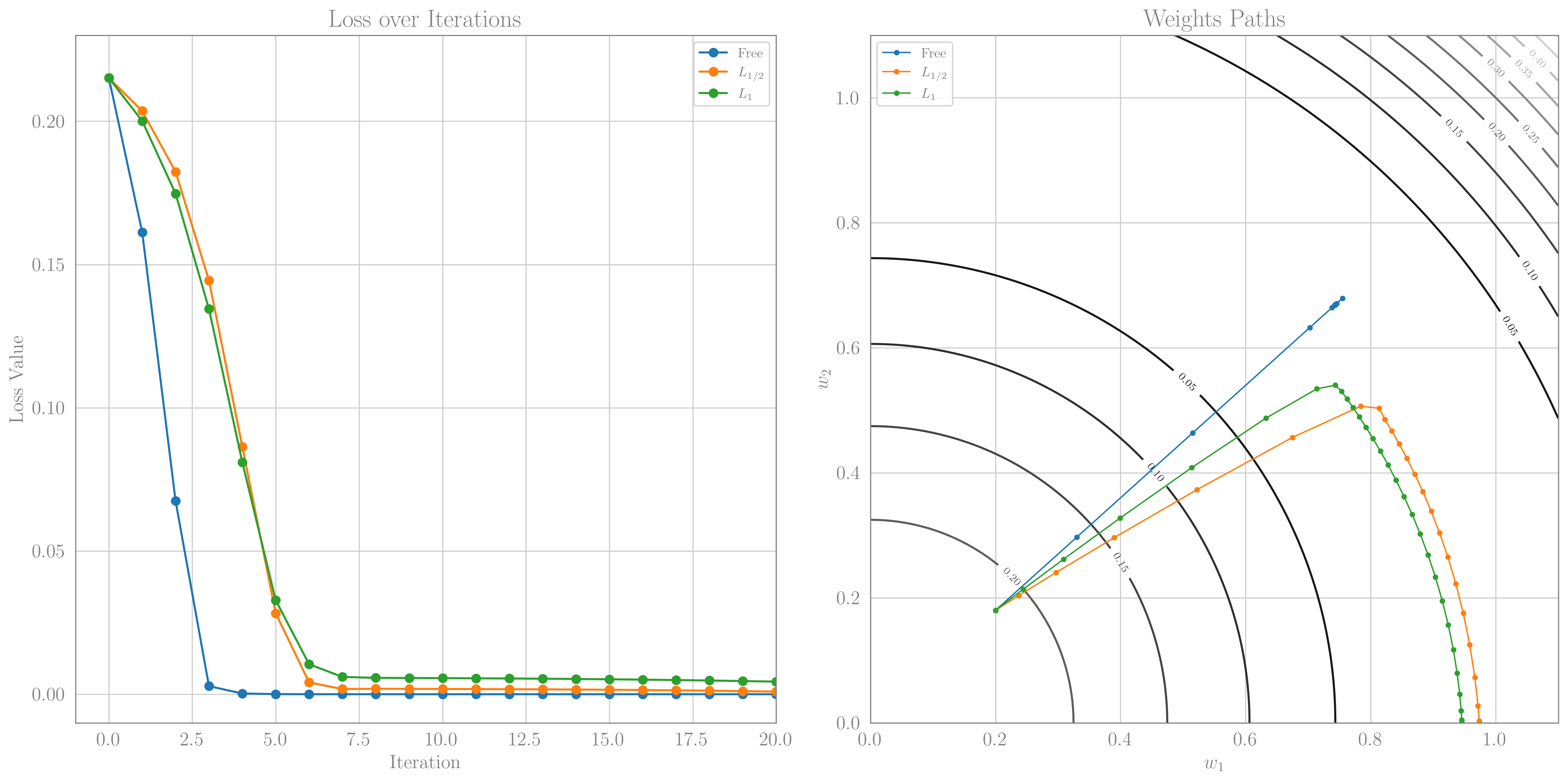 Numerical gradient decent in the ‘Higgs Potential’ for the unregulated case, and using $L_p$ norms. Left: The evolution of the loss. Right: The trajectories of the weight on the loss surface in the presence of different regularizations. We see in both the $p=1/2$ and $p=1$ case that indeed one of the weights is pushed to 0. In both cases, we also see that the weights first try to get to the minimal loss surface (a circle of radius 1), and only then travel towards the sparse solution.
PAdam: the $L_p$ Adam Optimizer
At this point, we have all the ingredients we need to implement the $L_p$ Adam optimizer. The only modification from the previous section, is that instead of the gradient $g$ in the weight update rule Eq.[3], we will use the Adam update rule. This is very similar to the AdamW version of Adam, only here instead of the $L_2$ weight decay step, we will use the $L_p$ norm weight decay step. The PAdam update rule is given by
| 1 | $g_t \gets \nabla \ell_0$ |
| 2 | $m_t \gets \beta_1 \cdot m_{t-1} + (1 - \beta_1) \cdot g_t$ |
| 3 | $v_t \gets \beta_2 \cdot v_{t-1} + (1 - \beta_2) \cdot g_t^2$ |
| 4 | $\hat{m}_t \gets m_t / (1 - \beta_1^t)$ |
| 5 | $\hat{v}_t \gets v_t / (1 - \beta_2^t)$ |
| 6 | $\hat{w}_t \gets w_{t-1} - \eta \hat{m}_t / (\sqrt{\hat{v}_t} + \epsilon)$ |
| 7 | $w_t \gets \vert w_t\vert^{2-p}\hat{w}_t/(\vert w_t\vert^{2-p}+\eta p\lambda)$ |
Steps 1–6 follow the standard Adam update algorithm. As a reminder, $\eta$ is the learning rate, $\epsilon$ ensures numerical stability, and $\beta_1$ and $\beta_2$ are the exponential decay rates for the moment estimates of the gradient $g_t$, namely $m_t$ and $v_t$. Step 7 is our sole modification to Adam, introducing the $L_p$ norm weight update rule. The PyTorch implementation that follows is not the most aesthetically pleasing, nor the most efficient one. Currently, for simplicity, we will inherit from the Adam optimizer class and append step 7 after the optimizer step. This approach avoids rewriting the entire optimizer, which is highly optimized, by adding a computationally inexpensive step. It’s important to note, however, that step 7 requires the weight before the Adam step, denoted $\vert w_t\vert$. To facilitate this, we must store all parameters before the optimizer step and then apply the decay to the parameters afterward. In principle, one could replace $\vert\hat{w}_t\vert$ instead of $\vert{w}_t\vert$ in step 7, which would be more memory-efficient and cleaner code, but this approach appears to yield inferior results. Bearing all this in mind, here is PAdam:
1
2
3
4
5
6
7
8
9
10
11
12
13
14
15
16
17
18
19
20
21
22
23
24
25
26
27
28
29
30
31
class PAdam(torch.optim.Adam):
    def __init__(self, params, lr=1e-3, betas=(0.9, 0.999), eps=1e-8, lambda_p=1e-2, p_norm=1, *args, **kwargs):
        super(PAdam, self).__init__(params, lr=lr, betas=betas, eps=eps, weight_decay=0, *args, **kwargs)
        self.p_norm = p_norm
        self.lambda_p = lambda_p

    @torch.no_grad()
    def step(self, closure=None):
        # Store the old params
        old_params = []
        for group in self.param_groups:
            old_params.append({param: param.data.clone() for param in group['params'] if param.grad is not None})

        # Perform the standard Adam step
        loss = super(PAdam, self).step(closure)

        # Perform the PAdam step
        for group, old_group in zip(self.param_groups, old_params):
            for param in group['params']:
                if param.grad is None:
                    continue

                # Use old parameters in the decay factor
                param_old = old_group[param]
                X = param_old.abs()**(2 - self.p_norm)
                update_term = X / (X + self.p_norm * group['lr'] * self.lambda_p)

                # Update the parameters
                param.data.mul_(update_term)

        return loss
First experiments on Fashion-MNIST
After this incredibly long build up, we are finally ready to test our new optimizer on a real-world dataset. We will use the Fashion-MNIST dataset, which is a dataset of 60,000 28x28 grayscale images of 10 fashion categories, along with a test set of 10,000 images. We used a relatively simple CNN with roughly 420k parameters. The network includes two convolutional layers of sizes 32 and 64, both followed by max-pooling, two dense layers with 128 and 10 units respectively, and a dropout rate of 0.2 applied after the activation function of the first dense layer. For improved performance, we normalized the dataset to have zero mean and unit variance and augmented the data by random rotations and translations. We note that the network used is very small compared to ones used in current literature (For e.g., about 11M parameters in ResNet18). This choice was made to make sure that the sparsity induced by PAdam is not simply compensating a very over-parametrized model.
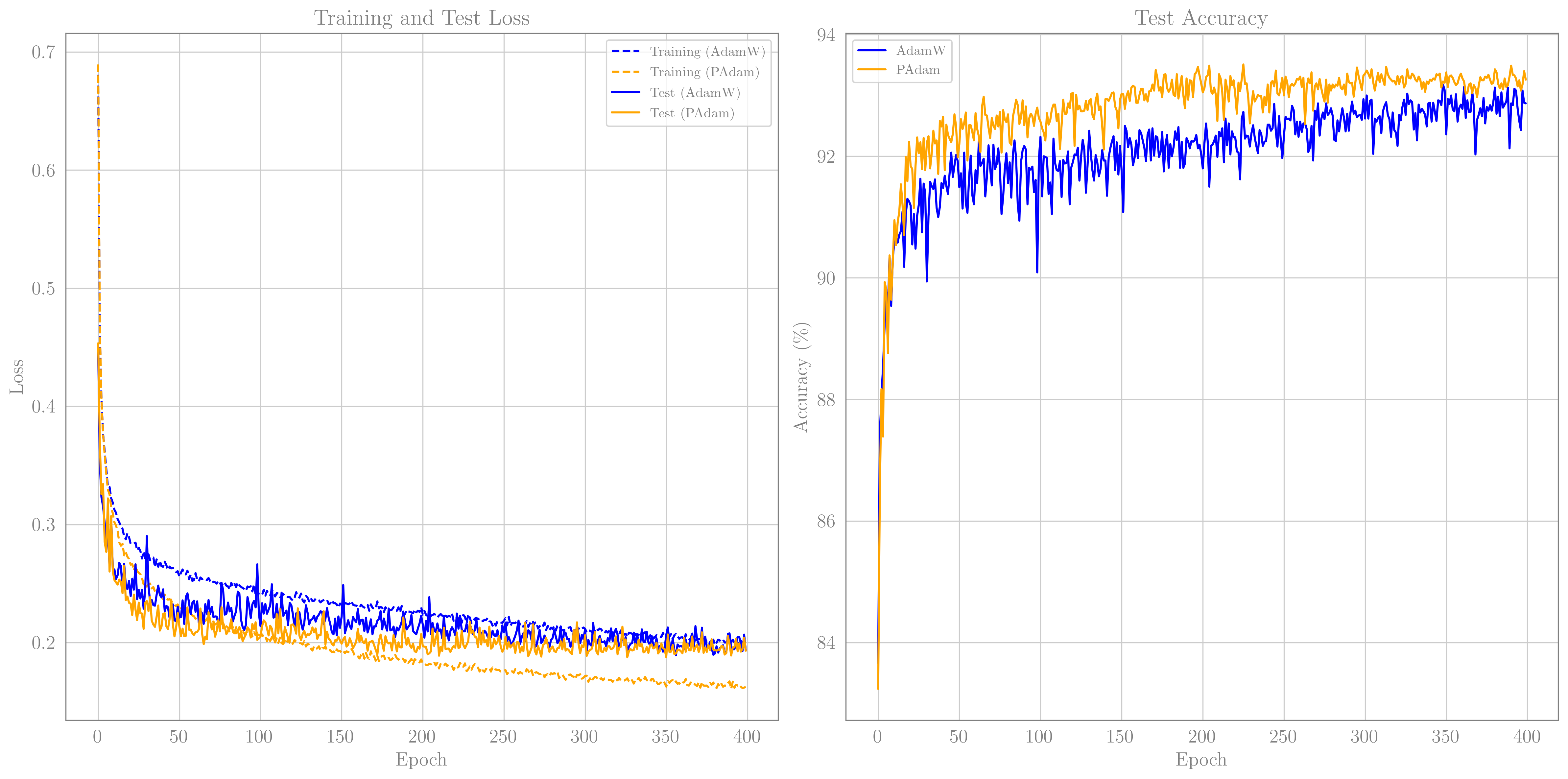
We trained the network for 400 epochs, once with AdamW optimizer, for $\lambda=0.1$, and once with PAdam, for $\lambda=0.003$ and $p=0.8$. For both we used an initial learning rate of $3\times 10^{-3}$, which decayed geometrically to $7.5\times10^{-4}$ during training. I did not systematically optimize the hyperparameters used. I did my best to find the best test accuracy for AdamW, and only then started plying with PAdam, which I was able to get to work quite similarly (even slightly better). Both optimizers reached about $93\%$ accuracy. The loss and accuracy is shown in the figure below
 Loss and accuracy curves for
 AdamW and PAdam, both resulted in very similar results.
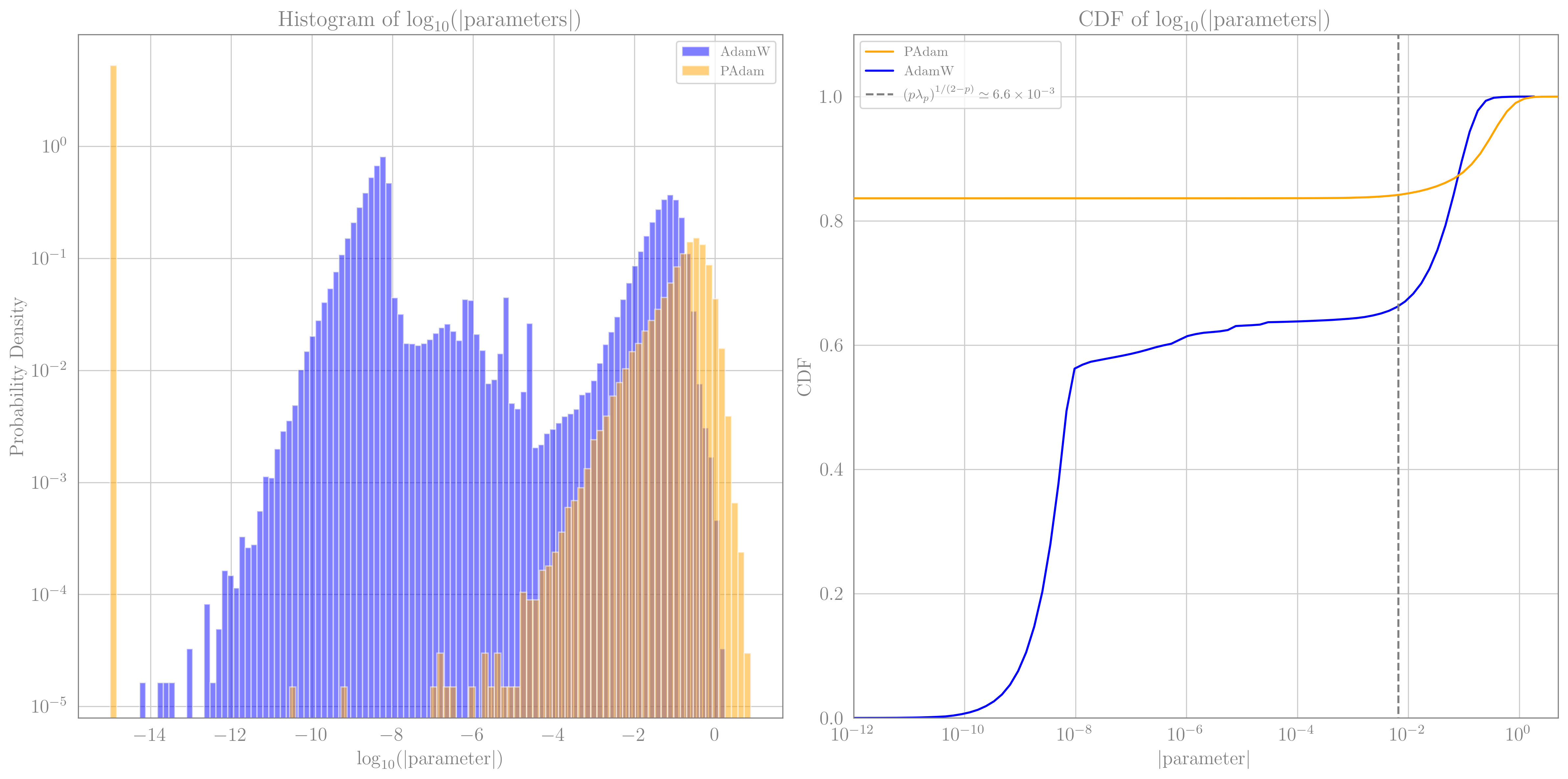
The more interesting result, is the level of sparsity PAdam obtained. In this specific examples, PAdam pushed $83.63\%$ of the weights to 0, whereas AdamW pushed only about $6.3\%$ below $10^{-9}$. This is a significant difference, which possibly could lead to reduced inference time, if treated correctly. Below we show the CDF of the absolute values of the weights, which shows nicely that for PAdam, practically all the non-vanishing weights are larger than $(p\lambda)^{1/(2-p)}\simeq6.6\times 10^{-3}$, which is the scale below which we expect to see a supression (c.f. Eq.[3]).
 Probability Density Function and Cumulative Density Function of the magnitude of weights for both
 AdamW and PAdam. The gray dashed line ont the right panel represent the value of $(p\lambda)^{1/(2-p)}$, below which PAdam is expected to suppress the weights.
Future directions and open questions
To finish off, I want to present some directions I wish to pursuit in the near future, some of which will be included in an upcoming paper.
Clearly one of this first things to do is to run larger, more complex, experiments. In the near future I will finish and possibly update this post with results from both ResNet trained on CIFAR, and hopefully will also a small transformer based model.
Large weight regularization
One thing to note about $L_{p<2}$ norms is that the regulator is stronger for smaller weights and weaker for larger ones. This is in contrast with the $L_{p>2}$ norm, which regulates larger weights more than smaller ones. Regulating only small weights seems problematic, as it will not address one of the core reasons regularization is used in the first place, namely, to avoid ‘dead neurons’ by penalizing large weights. Here are a few thoughts on how to regulate large weights in a PAdam-like optimizer.
Elastic net-like regularization: Much like elastic net [4] is a combination of $L_1$ and $L_2$ regularization, we can combine $L_2$ regularization with our suggested $p$-norm weight update. This is probably the simplest extension and the modified weight update rule will now be
\[w_i^{(t+1)}=\frac{\left\vert w_i^{(t)}\right\vert^{2-p}}{\left\vert w_i^{(t)}\right\vert^{2-p}(1+\eta\lambda_2)+\eta p\lambda_p}\left(w_i^{(t)}-\eta g_i^{(t)}\right)\]Preliminary experiments with this update rule seem to help at the early stages of learning.
$p$-scheduling: Just like any other hyperparameter, $p$ can be held fixed, or change its value as training evolve. Changing $p$ gradually from $2$ to it final $p<2$ value, will allow the network to first settle toward a desired minimum, and only then let the $p<2$-norm ‘look’ for sparser solutions. One advantage of $p$-scheduling over the elastic-net approach, is that weights that are initialized below the $p<2$-norm threshold will not get stuck at 0.
Departure from the adiabatic limit: One last possibility, is to make $\boldsymbol{s}$ a dynamical variable again. Initializing $\boldsymbol{s}=\mathbb{1}$ and forcing it learn slower than $\boldsymbol{w}$, will allow the network to initially learn in an $L_{2}$-like manner, but then slowly transition to the $L_{p<2}$ regime. This enjoys similar advantages to $p$ scheduling, but is more complex to implement, and will require some memory and computation overhead (though likely negligible).
References
[1]: Xu, Zongben et al. “$L_{1/2}$ regularization: a thresholding representation theory and a fast solver”
[2]: Chen, F., Shen, L. and Suter, B.W. “Computing the proximity operator of the $\ell_p$ norm with $0<p<1$”
[3]: O’Brien, Cian and Plumbley, Mark D. “Inexact Proximal Operators for $\ell_{p}$-Quasinorm Minimization”
[4]: Hui Zou, Trevor Hastie. “Regularization and Variable Selection Via the Elastic Net”